Automatic Report Generation Examples
Use hwCFDReport to create a .pptx or .pdf report with user defined visualization.
Create a Simple Input File
To create a simple input file with a cover page and summary, navigate to the simulation results folder, and create a file named report.img with the following contents:
COMMAND, followed by curly
braces {} with options specified inside the braces. The simulation
data to summarize is specified with the DATASET{}
command.DATASET{
resultFile = "uFX_fullData\uFX_output.case"
summary_file = " uFX_summary.txt"
summary_in_report = on
}
REPORT("Run summary"){
report_type = run_summary
format = pptx
}>> hwcfdReport –img report.imgAdd Images
IMAGE{} command to tell the utility to create and display an
image. In the command options, specify which parts are to be shown and the views
from which the image is to be rendered. In this example, we define two views: front
and left.IMAGE("Car_view"){
parts = {"Car"}
views = {"front","left"}
image_type = static
}PART{} command. This particular command instance is named
Car and is referenced above with this name. A PART{} command
includes all boundaries and default visualization settings. These are optional and
can be customized as seen
below:PART("Car"){
show_boundary_names = {"_all"}
display_type = solid
color_type = constant
constant_color = "white"
}
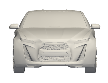 Figure 1. |
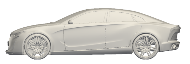 Figure 2. |
Results Visualization Tools
The advanced options enable you to unlock more colorful possibilities. Visualization
mainstays such as Contours, Cut-planes, Iso-surfaces, and Streamlines have dedicated
commands. Two- dimensional plots such as Line-plots and Bar-charts can also be
created. All these commands can be further customized using the
VARIABLE{} command that makes these commands more powerful and
portable across multiple simulations. Last but not the least, two simulation results
can be used to create a report that renders images side by side for a quick spot the
difference comparison.
Surface Contours
color_type from constant to contour. This changes the
coloring of the car model from a constant color to a surface contour. We also
specify the contour function which controls the coloring of the contour, in this
example time_avg_pressure_coefficient. This is followed by more
settings that control the legend on the right-hand corner in the
plot.IMAGE("Surface Cp"){
parts = {"Surface Cp"}
views = {"front_top_left"}
image_type = static
}
PART("Surface Cp"){
display_type = solid
solid_display_type = smooth
color_type = contour
contour_function = time_avg_pressure_coefficient
legend_display = on
legend_min = -0.5
legend_max = 0.5
}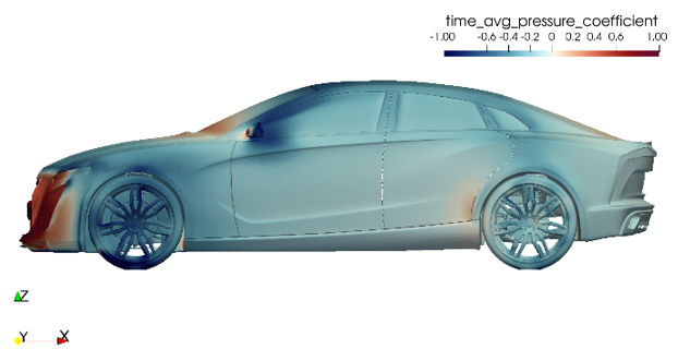
Figure 3.
Cut Planes
y = 0 is
defined. The instantaneous velocity magnitude, inst_velocity_mag,
is used to color the plane and the size of the plane is controlled by the inputs:
x_min, x_max, and z_max.car_length and
car_height are needed for the command to
work.IMAGE("Cut plane y inst. vel"){
cut_planes = {"y cut vel_inst"}
parts = {"Full vehicle - white"}
views = {"left"}
clip_parts = off
}
CUT_PLANE("y cut vel_inst"){
normal_direction = y
cut_location = 0.0
color_type = contour
contour_function = total_pressure_coefficient
legend_display = on
legend_min = 0.0
legend_max = 45.0
x_min = -0.78 - car_length/4.0
x_max = 3.29 + car_length
z_max = 1.3 + 0.5*car_height
}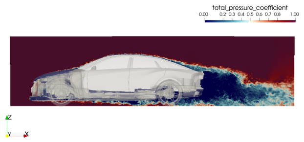
Figure 4.
Variables
variable_name, and an expression associated
with it. The expression can be a constant, another variable, or a mathematical
expression containing more variables. The following variables,
car_length and car_height need to be defined
to get the CUT_Plane{} in the previous section to work
correctly.VARIABLE{
variable_name = car_length
expression = 4.07
}
VARIABLE{
variable_name = car_height
expression = 1.317
}Iso-Surfaces
ISO_SURFACE{} command. In this
example, the time averaged pressure coefficient,
time_avg_pressure_coefficient, is used to create the
iso-surface which is then colored with a constant color, blue for
time_avg_pressure_coefficient=-0.3 and red for
time_avg_pressure_coefficient=0.5.
IMAGE("Cp Iso""){
parts	= {"Full vehicle - white"}
iso_surfaces	= {"Cp = -0.3”,” Cp = 0.5"”}
views	= {"left"}
image_type	= static
}
ISO_SURFACE("Cp = -0.3"){
iso_function	= time_avg_pressure_coeffient
iso_value	= -0.3
display_type	= solid
solid_display_type	= smooth
color_type	= constant
constant_color            = blue
}

ISO_SURFACE("Cp = 0.5"){
iso_function	= time_avg_pressure_coeffient
iso_value	= 0.5
display_type	= solid
solid_display_type	= smooth
color_type	= constant
constant_color            = red
}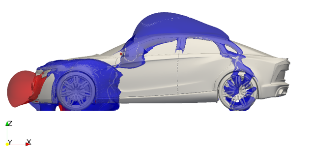
Figure 5.
Line Plots
data_file input. The data in the
ASCII file is organized
into rows and columns. Specify the column numbers in the x_column
and y_column fields to get a line
plot.LINE_PLOT("Instantaneous drag"){
data_source = "file"
data_file = "./uFX_coefficientsData/uFX_coefficients_Inst.txt"
num_header_rows = 11
x_column = 1
y_columns = {2}
x_label = "Time (s)"
y_label = "Coefficients"
title = "Instantaneous Drag"
legend_labels = "C_d"
show_legend = on
show_grid = on
}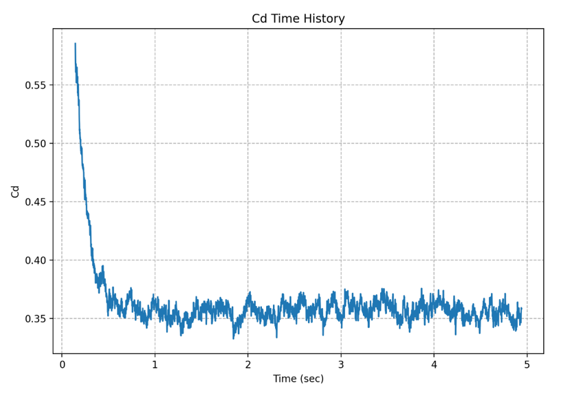
Figure 6.