Adaptive solver: operating mode in 3D
An example in magnetostatic 3D
You can use this new functionality with a 3D magnetostatic example, available from the supervisor. In the Open example context:
| Step | Description | Illustration |
|---|---|---|
| 1 |
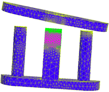
For this example, you can start from the mesh carried out by the aided mesh. By definition, this mesh is « non-adapted » to the physics of the problem. |
|
| 2 |
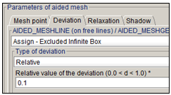
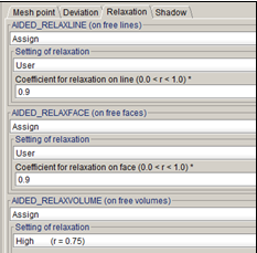
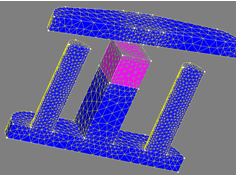
To observe the local impact of the adaptive solving, start from an aided loose mesh such as:
|
|
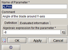
| 3 | Modify the angle of the blade around Y-Axis: [ALPHA] = -8° |
|
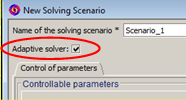
| 4 | To activate the adaptive solver, the user must select Adaptive solver in the scenario that he has created. |
|
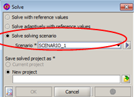
| 5 | The user solves this scenario by opening the dialog box Solve, which exists in the Solving menu and by selecting Solve solving scenario |
|
| 6 |
Modify the Adaptive solver options:
|
|
| 7 |
User threshold (0.0 < s <= 1): 0.1 Maximum number of iterations: 4 Volume regions to be excluded: none. |
|