Constraints
Introduction
In the data tree of Flux the node Solver > Optimization > Constraints allows
the user to define some constraints which are structural or physical limitations
imposed by the optimizer, a constraint allow the user to control the shape of the
design with some symmetries constraints, volume values constraints or physical
limits. The short list of the constraints is given below:
| Constraints | Required information |
|---|---|
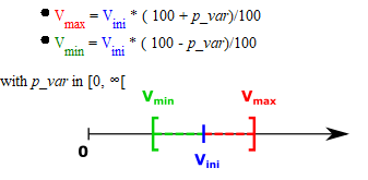
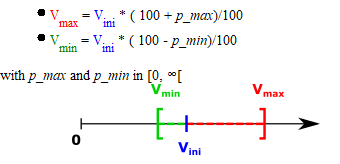
| Physical constraint |
|
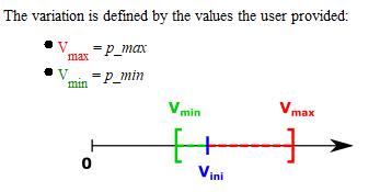
| Constraints on 2D faces volume |
|
| Symmetry constraint (defined by direction) |
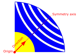 Figure 4. Origin point and a simple symmetry axis over the rotor of a rotating machine |
| Symmetry constraint (defined by angle) |
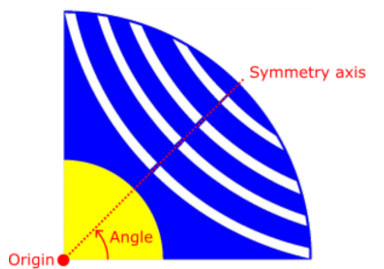 Figure 5. Origin point and a simple symmetry axis over the rotor of a rotating machine |
| Double symmetry constraint (defined by direction) |
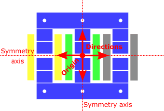 Figure 6. Origin point and double symmetry axis over an electromagnetic device |
| Double symmetry constraint (defined by angle) |
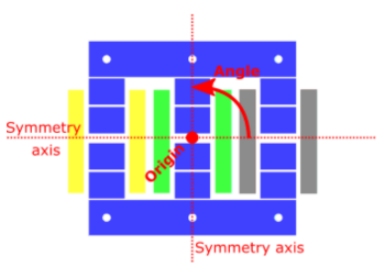 Figure 7. Origin point and double symmetry axis over an electromagnetic device |