Nonlinear finite element analyses confront users with many choices. An understanding of the fundamental concepts of
nonlinear finite element analysis is necessary if you do not want to use the finite element program as a black box.
The purpose of this manual is to describe the numerical methods included in Radioss.
The historical shell element in Radioss is a simple bilinear Mindlin plate element coupled with a reduced integration scheme using one integration point.
It is applicable in a reliable manner to both thin and moderately thick shells.
Beam type /PROP/TYPE18 uses a shear beam theory or Timoshenko formulation like /PROP/TYPE3, but the section inputs (area, inertia) can be default values and can also be discretized by sub-sections; numerical
integrations are used to calculate internal forces.
Kinematic constraints are boundary conditions that are placed on nodal velocities. They are mutually exclusive for each degree
of freedom (DOF), and there can only be one constraint per DOF.
The stability of solution concerns the evolution of a process subjected to small perturbations. A process is considered
to be stable if small perturbations of initial data result in small changes in the solution. The theory of stability
can be applied to a variety of computational problems.
A large variety of materials is used in the structural components and must be modeled in stress analysis problems.
For any kind of these materials a range of constitutive laws is available to describe by a mathematical approach the
behavior of the material.
Explicit scheme is generally used for time integration in Radioss, in which velocities and displacements are obtained by direct integration of nodal accelerations.
The performance criterion in the computation was always an essential point in the architectural conception of Radioss. At first, the program has been largely optimized for the vectored super-calculators like CRAY. Then, a first parallel
version SMP made possible the exploration of shared memory on processors.
Three coordinate systems are introduced in the formulation:
Global Cartesian fixed system
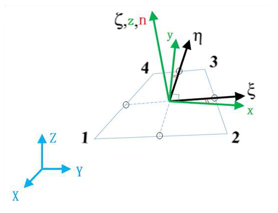
 X=(X→i+Y→j+Z→k)
Natural system (ξ,η,ζ), covariant axes x,y
Local systems (x, y, z) defined by an orthogonal set of unit base vectors (t1, t2, n). n is taken to be normal to the mid-surface coinciding with ζ, and (t1, t2) are taken in the tangent plane of the mid-surface.
Figure 1. Local Reference Frame
The vector normal to the plane of the element at the mid point is defined
as:(1)
n=x×y‖x×y‖
The vector defining the local direction is:(2)
t1=x‖x‖
Hence, the vector defining the local direction is found from the cross product of the two
previous vectors:(3)