ACU-T: 1000 HyperMesh CFD UI Introduction
This tutorial introduces you to the workflow for setting up a Computational Fluid Dynamics (CFD) analysis using Altair HyperMesh CFD. HyperMesh CFD is a powerful tool which provides a single, streamlined platform for performing a CFD analysis, starting from importing CAD through post-processing results. In this tutorial, you will learn how to use HyperMesh CFD for setting up a CFD analysis while exploring different capabilities available within the software for importing a geometric model, validating the geometry, setting up simulation parameters and boundary conditions, and generating a mesh. You will then launch AcuSolve simulation directly from HyperMesh CFD and post-process the results using HyperMesh CFD Post.
Prerequisites
To run this simulation, you will need access to a licensed version of HyperMesh CFD and AcuSolve.
Analyze the Problem
An important step in any CFD simulation is to examine the engineering problem at hand and determine the important parameters that need to be provided to AcuSolve. Parameters can be based on geometrical elements, such as inlets, outlets, or walls, and on flow conditions, such as fluid properties, velocity, or whether the flow should be modeled as turbulent or as laminar.

Figure 1. Schematic of the Problem
Introduction to HyperMesh CFD
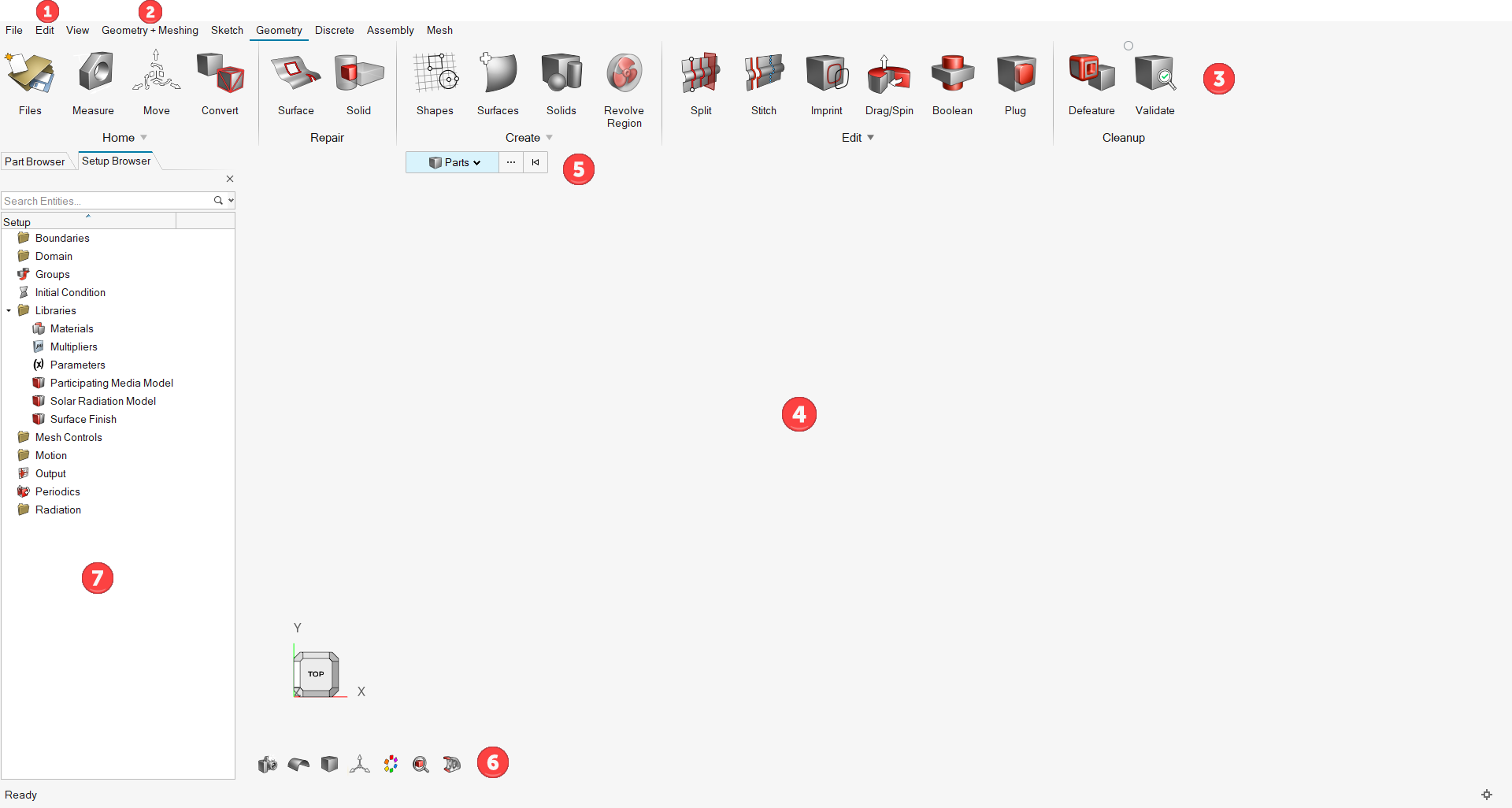
Figure 2.
The HyperMesh CFD graphical user interface can be divided into six general categories as shown in the figure above.
- The menu bar contains the drop-down menus for File input-output, Edit, and View operations.
- The modeling environment switcher is used to populate relevant ribbons and tools based on modeling tasks.
- Ribbons contain various functionalities and tools available
in HM-CFD. Navigate between various ribbons by clicking the ribbon tabs to the right
of the modeling environment switcher. After selecting a ribbon, the corresponding
tool icons are displayed on the screen. The functionalities of various ribbons and
corresponding tools are briefly explained in this section.
- Sketch ribbon
- The Sketch ribbon provides multiple ways to define sketching plane
by selecting planes aligned with global coordinate systems. You can
also get references of existing geometry by cutting geometry or
projecting geometry to a plane. It provides capabilities to create
sketches using multiple interactive tools. A dimensioning capability
enables you to parametrize dimensions of sketches. One of big use
case for CFD is to get cutting lines of rotating geometry and create
a non–cylindrical axisymmetric MRF region around them.
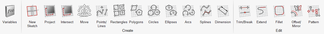
Figure 3. - Geometry ribbon
-
The Geometry ribbon consists of tools for repairing, creating, editing, and validating the geometry.
When a geometry file is imported, the Repair tools can be used to detect any defects present in the CAD model like intersections, free edges, duplicates, sliver surfaces, and so on and fix those errors.
The tools available under the Create sub-section can be used to create geometric entities like points, lines, surfaces, and solids.
The tools required for performing operations like plugging cavities, stitching surfaces, and so on are available under the Edit sub-section.
The Defeature tool can be used to resolve defects or model a new geometry, while the Validate tool can be used to detect any defects present in the CAD model. This process is usually known as CAD cleanup.
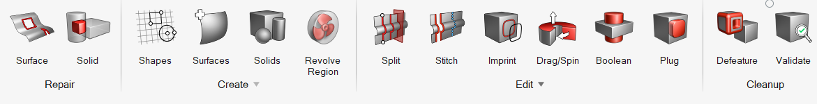
Figure 4. - Discrete ribbon
-
The Discrete ribbon consists of tools used for working with FE geometry. You can cap openings, connect geometry, define local or proximity-based wrap controls, wrap the model, remesh the wrapped results, and fix the mesh quality.
-
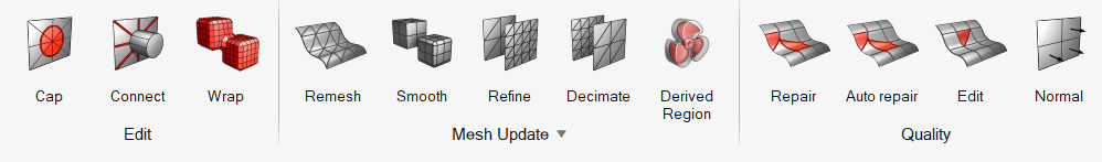
Figure 5. - Assembly ribbon
- The Assembly ribbon is useful for finding, managing, and organizing the parts in your model.
-
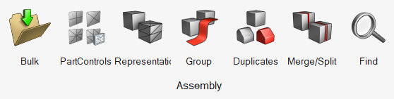
Figure 6. - Flow ribbon
-
The Flow ribbon contains tools for setting up simulation parameters, solver settings, and reference properties such as material properties, heat sources, porous media, and so on. The Setup sub-section is where you set up the physics equations and solver settings as well as create material models, multiplier functions, and parameters.
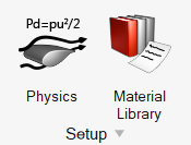
Figure 7.The Domain sub-section contains tools for assigning reference properties such as materials, heat and momentum sources, and reference frames to volumes.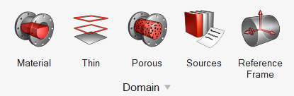
Figure 8.Surface boundary conditions such as inlets, outlets, and far fields, can be assigned using the tools under the Boundaries sub-section. By default, all the surfaces are assigned a boundary condition of type ‘auto_wall’ and are placed under Default wall. Refer to the AcuSolve Surface Processing manual for more information about auto_wall. As you assign boundary conditions to the surfaces, they are moved into the respective group.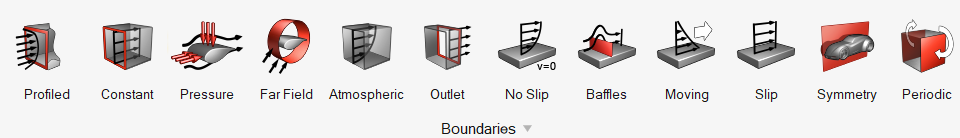
Figure 9. - Radiation ribbon
-
The Radiation ribbon is where you define radiation physics, create thermal, solar, and participating media models, and apply radiation parameters.
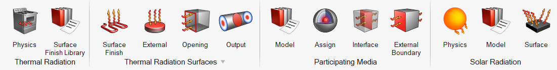
Figure 10. - Motion ribbon
-
Mesh boundary conditions and mesh-motion-related parameters can be defined using the tools available in the Motion ribbon. Parameters such as mesh motion type and mesh displacement constraints can be defined here. In addition to the mesh boundary conditions, code coupling with external codes such as OptiStruct and MotionSolve can be defined here
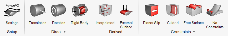
Figure 11. - AcuTrace ribbon
- The AcuTrace ribbon computes particle
traces as a series of segments solving particle motion. It computes
traces for unsteady as well as steady flow fields, for flows with
mesh motion as well as without, and for flows computed on meshes
with interface surfaces. To solve a problem with AcuTrace, you must first run AcuSolve. You can set up for finite mass and
massless particles.
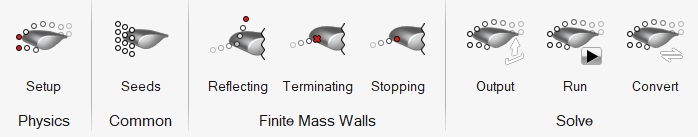
Figure 12. - Mesh ribbon
-
Meshing parameters such as surface mesh controls, boundary layer parameters, volume mesh parameters, and zone meshing parameters can be defined here. This ribbon also has tools for local remeshing. Once all the mesh controls are defined, you can generate the mesh using the Volume tool.
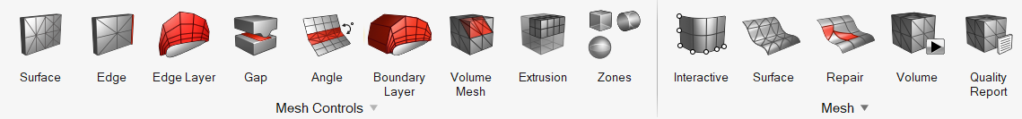
Figure 13. - Aerodynamics and Aeroacoustics Setup
- The setup ribbon is used carry out external aerodynamics and fan
noise simulations with the ultraFluidX
solver.

Figure 14. - Solution ribbon
-
The Solution ribbon is used to set up monitors for any individual point, surface, or volume set output. The Field tool is used to set the nodal output frequency for the entire model. The Initialize tools are used to set the nodal initial conditions for variables like pressure, velocity, and variables specific to each turbulence model.
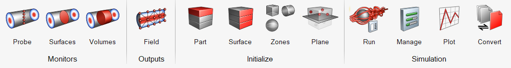
Figure 15.Once the complete set up is done, the Run tool is used to launch AcuSolve. Once the AcuSolve run parameters are set, the simulation can be started, and you can monitor the status of the run using the run manager.
- Post ribbon
- The Post ribbon is where you can post-process the results. The
Visualize tools under the Post ribbon can be used to create things
like plots, streamlines, iso surfaces, and section cuts. The
Measures tools can be used to probe variables at desired
locations.
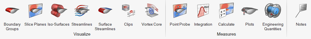
Figure 16. - Morphing Ribbon
- The Morphing ribbon is used to morph mesh or FE geometry. You can define constraints to fix some nodes or define relative movement.
- Once morphing is done, you can create shapes and design variables
using the “Shape” tool and submit DOE studies using “DOE Study”
tool.
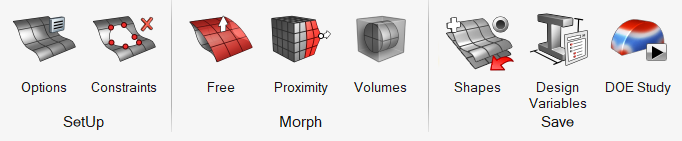
Figure 17.
- The modeling window is where the
model is displayed. The model display can be manipulated using the view controls
shown in the table below. Clicking on the model will highlight the entity being
selected and right-clicking on an entity will give you additional options for the
operations that can be done based on the context. Some of the functions available
using right-click are Show, Hide, Isolate, Select, Advanced select, Create groups,
and so on.
Button Operation Middle mouse scroll Zoom in and out Right-click hold and drag Pan the model Middle mouse click hold and drag Rotate the model Left-click Select entity Ctrl + Left-click Select multiple entities Left-click hold and drag Window select Shift + Left-click Deselect entities - The entity selector enables you to
control what entities can be selected using the left-mouse button. The selector can
be set to any of the entities shown in the figure below. When you open any tool, the
selector is automatically set to the entity (entities) which are appropriate for
that command.
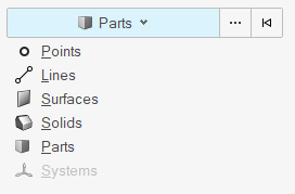
Figure 18. - The visualization of the model can be controlled using the tools available in
View Controls toolbar. The display of mesh, model
coloring, section cuts, standard views, and so on can be controlled using these
tools.

Figure 19. - The browsers show the entities and setup parameters in the model and list them in a tree structure. They can be turned on or off from the View menu. Some common functions that can be performed in all browsers are show, hide, and isolate.
Start HyperMesh CFD and Create the HyperMesh Model Database
-
Create a new .hm database in
one of the following ways:
- From the menu bar, click .
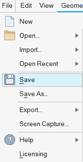
Figure 20. - From the Home tools, Files tool group, click the Save As tool.
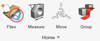
Figure 21.
- From the menu bar, click .
Import and Validate the Geometry
Import the Geometry
-
In the Geometry Import Options dialog, leave all the
default options unchanged then click Import.
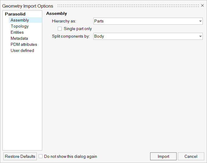
Figure 22. -
Once the geometry is loaded, rotate and observe the features of the model.
The view of the model displayed in the modeling window can be controlled using the following view controls.
Button View Control Middle mouse scroll Zoom in and out Right-click hold and drag Pan the model Middle mouse click hold and drag Rotate the model 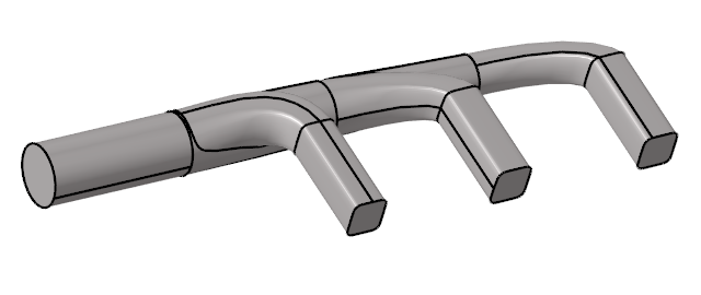
Figure 23.
Validate the Geometry
-
From the Geometry ribbon, click the Validate tool.

Figure 24.The Validate tool scans through the entire model, performs checks on the surfaces and solids, and flags any defects in the geometry, such as free edges, closed shells, intersections, duplicates, and slivers.The current model does not have any of the issues mentioned above. Alternatively, if any issues are found, they are indicated by the number in the brackets adjacent to the tool name.
Observe that a blue check mark appears on the top-left corner of the Validate icon. This indicates that the tool found no issues with the geometry model.
Figure 25.
Set Up the Problem
Set Up the Simulation Parameters and Solver Settings
-
From the Flow ribbon, click the Physics tool.

Figure 26.The Setup dialog opens. -
Under the Physics models setting:
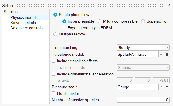
Figure 27. -
Click the Solver controls setting and verify that the
parameters are set as shown in the figure below.
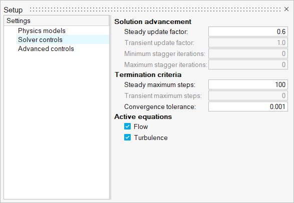
Figure 28.
Assign Material Properties
-
From the Flow ribbon, click the Material tool.

Figure 29. -
From the modeling window, click anywhere on the
manifold.
The entire manifold geometry is highlighted and a Material microdialog appears.
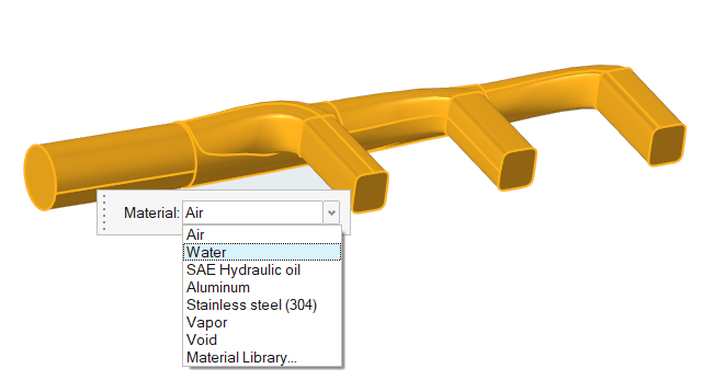
Figure 30. -
On the guide bar, click
 to execute the command.
The changes made in the tool are not effective until they are executed by clicking the icon.Once the command is executed, the color of the geometry changes to indicate the material assigned to the volume. In this case, there is only one volume in the geometry so there is a single color. Alternatively, if there are multiple volumes with different materials assigned, the model will be displayed accordingly with distinct colors for each material assigned.
to execute the command.
The changes made in the tool are not effective until they are executed by clicking the icon.Once the command is executed, the color of the geometry changes to indicate the material assigned to the volume. In this case, there is only one volume in the geometry so there is a single color. Alternatively, if there are multiple volumes with different materials assigned, the model will be displayed accordingly with distinct colors for each material assigned.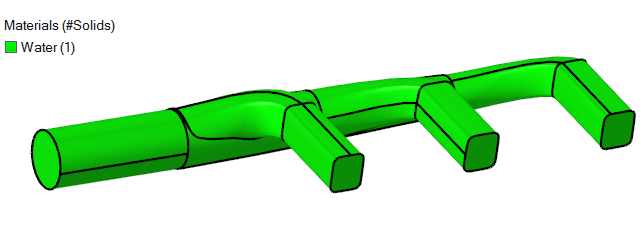
Figure 31. -
On the guide bar, click
 to exit the
tool.
to exit the
tool.
Assign the Flow Boundary Conditions
The current model has one inlet, three outlets, and walls for the rest of the surfaces. When a geometry model is imported into HyperMesh CFD, all the surfaces are placed in the Default Wall (i.e. Type = auto_wall). As you start assigning the surface boundary conditions, those surfaces are moved into a new boundary condition group. All the surface boundary condition tools are placed under the Boundaries sub-section of the Flow ribbon.
-
From the Flow ribbon, Profiled
tool group, click the Profiled Inlet tool.

Figure 32. -
In the modeling window, click the surface of the
inlet.
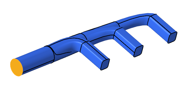
Figure 33.Observe that a new group named "Inlet" is created under the Boundaries list in the top-left corner of the modeling window. Once the current command is executed, the highlighted surface will be moved into the Inlet group. -
In the microdialog, enter a value of
2.0 m/sec for Average velocity.
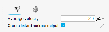
Figure 34. -
On the guide bar, click
to execute the command.
The color of the inlet surface in the modeling window is updated.Note: The color assigned to the surfaces is random. Therefore, the color of the surfaces shown in the images below might be different from what you see on your screen.
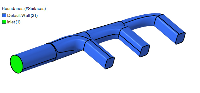
Figure 35. -
Click the Outlet tool.

Figure 36. -
Click the three outlet surfaces shown in the figure below.
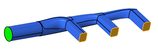
Figure 37. -
Leave the default options in the dialog unchanged then click
on the guide bar to execute the command.
The color of the outlet surfaces change and the list of boundaries on the left are updated. The number of surfaces under each group are shown in the brackets.
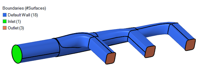
Figure 38.Note:- To update the color of any group, click on the colored-square on the left of the group name and select the color of your choice from the palette.
- To update the name of any group, right-click on the group name and select Rename from the context menu.
-
On the guide bar, click to exit the
tool.
Define Mesh Controls
Now that you have assigned the material properties and boundary conditions, you will define the meshing parameters for the model and then generate the mesh.
Define the Surface Mesh Controls
-
From the Mesh ribbon, click the Surface tool.

Figure 39. -
Right-click in the modeling window and go to .
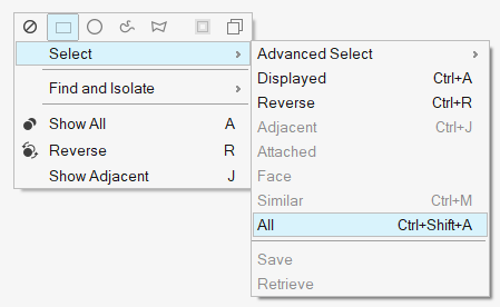
Figure 40.All the surfaces in the model are highlighted and a dialog for surface mesh parameters appears. -
Enter 0.003 m for the Average element size.
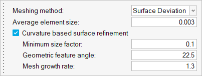
Figure 41. -
Leave the default values for the remaining parameters unchanged then click
on the guide bar to execute
the command.
Define the Boundary Layer Mesh Parameters
-
From the Mesh ribbon, click the Boundary Layer tool.

Figure 42. -
Right-click in the modeling window and go to .
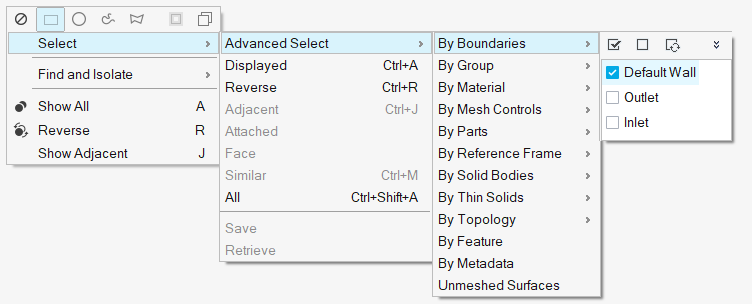
Figure 43.All the wall surfaces are highlighted and a dialog for boundary layer parameters appears. -
Enter the values in the dialog as shown in the figure below.
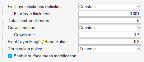
Figure 44. -
On the guide bar, click
to execute the command.
Generate the Mesh
-
From the Mesh ribbon, click the
Volume tool.

Figure 45. -
In the Meshing Operations dialog, enter an Average element
size of 0.005 m.
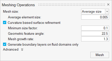
Figure 46. -
Click Mesh.
Once the meshing process has started, the Run Status dialog appears. To view the status of the meshing process, right-click on the process row and select View log file.Once the meshing is done, the run status is updated accordingly, and you are automatically moved to the Solution ribbon.
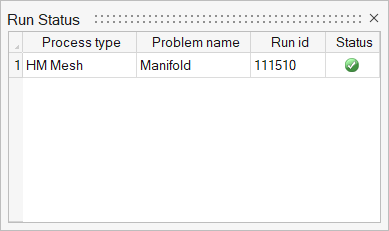
Figure 47.
Run AcuSolve
-
From the Solution ribbon, click the Run tool.

Figure 48. -
Leave the remaining options as default and click
Run to launch AcuSolve.
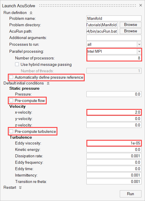
Figure 49.The Run Status dialog opens again and the AcuSolve run appears on the list. -
Right-click on the AcuSolve run and select
View log file.
A summary of the run printed in the dialog indicates that AcuSolve has finished running the simulation. Once the solution is converged, the Status will be updated accordingly.
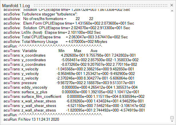
Figure 50. -
In the Run Status dialog, right-click on AcuSolve run and select Plot time
history to launch the Plot Manager.
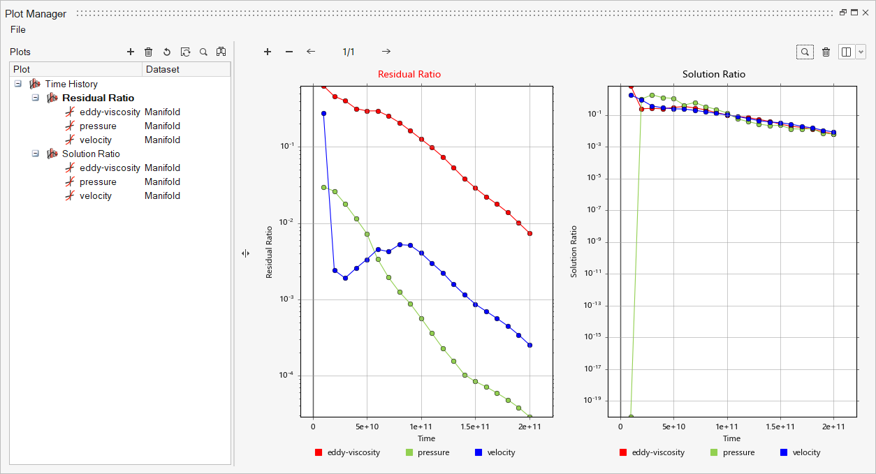
Figure 51.The above plot shows the residual and solution ratios of the equations as the solution progresses through each time step. The convergence check is performed on the residual and solution increment ratios of each equation in the problem. For the residual, the ratio of the residual norm over the norm of the forces of the systems is used. For the solution increment, the ratio of the solution increment norm over the solution norm is used. These ratios are computed separately for each solution field, such as pressure and velocity.
Once the pressure and velocity residual ratios reach a value less than the specified convergence tolerance (0.001), the solution is considered to be converged. By default, the eddy viscosity convergence tolerance is set to a magnitude of one order higher than the specified convergence tolerance (0.01).
Once the pressure and velocity solution ratios reach a value less than the specified convergence tolerance (0.01), the solution is considered to be arrived at steady state. The eddy viscosity solution ratio convergence tolerance is set to a magnitude of one order higher than the specified solution ratio convergence tolerance (0.1).
Post-Process the Results with HyperMesh CFD Post
This part of the tutorial shows you how to work with a steady state solution using HyperMesh CFD Post.
Load the Results
Create Pressure Contours on Boundary Surfaces
-
Click the Boundary Groups tool.

Figure 52. -
Select all surfaces in the model by holding the left mouse button, dragging,
and drawing a rectangle across the manifold.
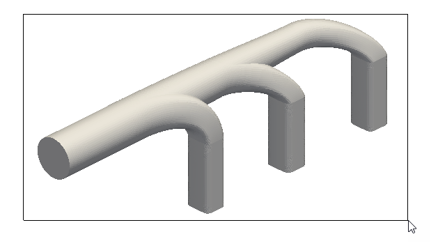
Figure 53. -
Activate the Legend toggle and click
 to reset the range.
-
Click
 and set the Colormap Name to Rainbow
Uniform.
and set the Colormap Name to Rainbow
Uniform.
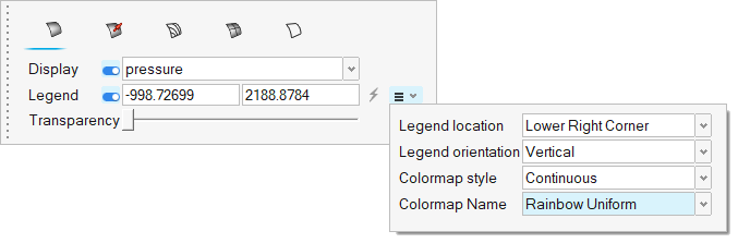
Figure 54. -
Click on the guide bar.
The pressure legend is in Pa.
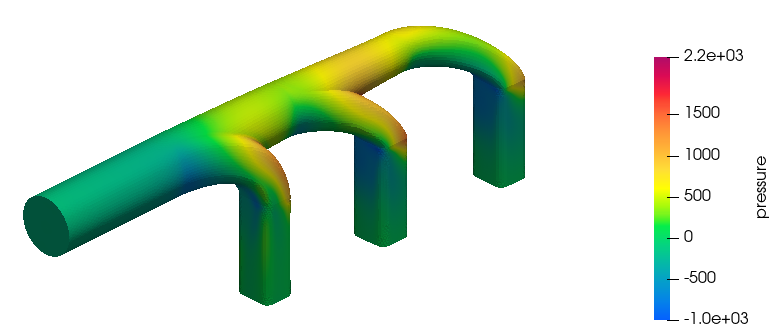
Figure 55.
Plot Velocity and Pressure Contours on a Section Cut
-
In the Post Browser, turn off the display of the boundary
surfaces by clicking on the icon next to Flow Boundaries.
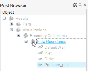
Figure 56. -
Click the Slice Planes tool.

Figure 57. -
Select the x-z plane in the modeling window.
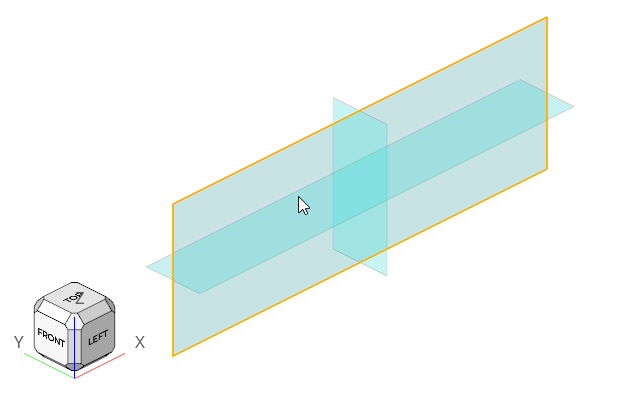
Figure 58. -
In the microdialog, click
 to adjust the plane with the Vector tool.
-
In the Vector tool dialog, click
 to
define the coordinates of the center of plane. Set the value of Y to
-0.015 and press Enter.
to
define the coordinates of the center of plane. Set the value of Y to
-0.015 and press Enter.
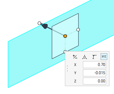
Figure 59. -
In the slice plane microdialog, click
 to
create the slice plane.
to
create the slice plane.
-
Activate the Legend toggle and click to reset the range.
-
Click and set the Colormap Name to Rainbow
Uniform.
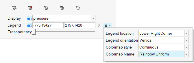
Figure 60. -
Click on the guide bar.
The pressure legend is in Pa.
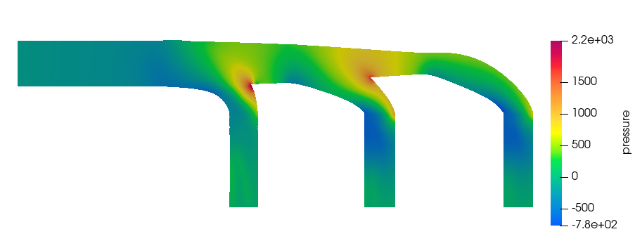
Figure 61. -
In the microdialog, change the Display variable to
velocity (m/s) then click on the
guide bar.

Figure 62.
Summary
In this tutorial, you worked through a basic workflow to carry out a CFD simulation and post-process the results using HyperMesh CFD. You started by importing the geometry and meshing the model in HyperMesh CFD. You also set up the model and launched AcuSolve directly from within HyperMesh CFD. Upon completion of the solution by AcuSolve, you post-processed the results in the Post ribbon. You learned how to create contours on the boundary surfaces and section cuts.