HL-T: 1050 Spot Weld (CBAR)

In this tutorial you will:
  • Import a model to HyperLife
  • Select the Weld module and define its required parameters
  • Create a material and assign it to the welds and sheet groups
  • Assign load histories for scaling the stresses from FEA subcases
  • Evaluate and view results
Before you begin, copy the file(s) used in this tutorial to your working directory.

Import the Model

  1. From the Home tools, Files tool group, click the Open Model tool.


    Figure 1.
  2. From the Load model and result dialog, browse and select HL-1050\Rail_SpotWeld.h3d for the model file.
    Note: The .h3d file should contain the following result types for this calculation:
    • CBAR/CBEAM Axial Force A
    • CBAR/CBEAM Shear Plane - 1A
    • CBAR/CBEAM Shear Plane - 2A
    • CBAR/CBEAM Torque A
    • CBAR/CBEAM Bending Plane - 1A
    • CBAR/CBEAM Bending Plane - 2A
    • CBAR/CBEAM Bending Plane - 1B
    • CBAR/CBEAM Bending Plane - 2B
    The Load Result field is automatically populated. For this tutorial, the same file is used for both the model and the result.
  3. Click Apply.


    Figure 2.

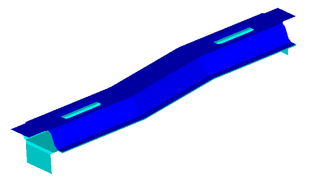
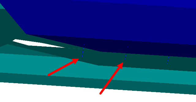
    The spot welds are modelled with CBAR elements between the two plates.


    Figure 3.
Tip: Quickly import the model by dragging and dropping the .h3d file from a windows browser into the HyperLife modeling window.

Define the Fatigue Module

  1. Click the arrow next to the fatigue module icon and select the Weld tool from the list of options.


    Figure 4.
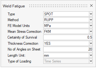
    The Weld dialog opens.
  2. Accept the default parameters.


    Figure 5.
  3. Exit the dialog.

Assign Materials

  1. Click the Material tool.


    Figure 6.
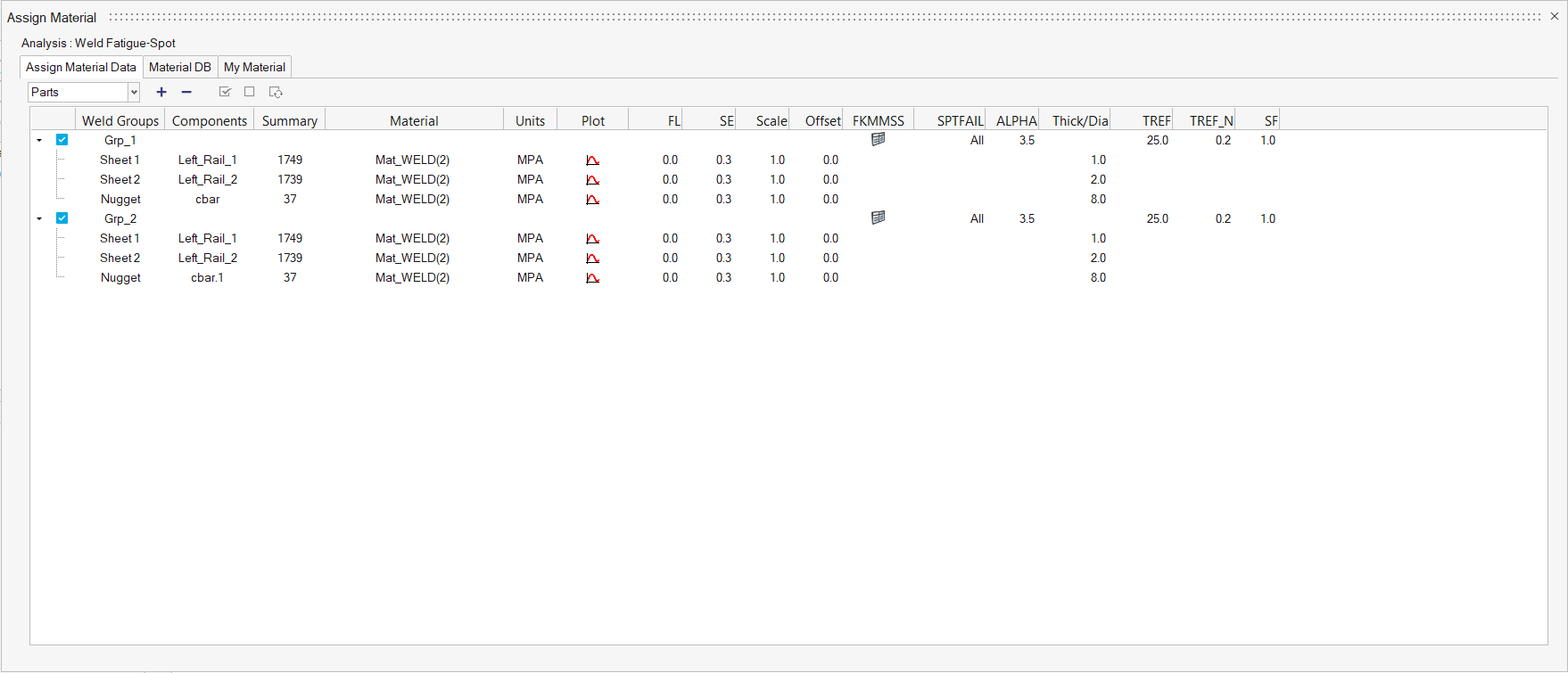
    The Assign Material dialog opens.
  2. Activate the checkboxes for the Grp_1 and Grp_2 sheet groups.
  3. Click the My Material tab.
  4. Click .
    A new material named Mat_WELD("n") is created.
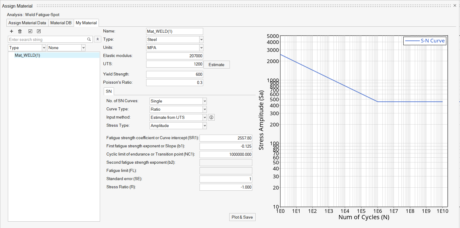
  5. Select Estimate from UTS as the input method.
  6. Select Steel as the type and enter a value of 1200 for UTS.
  7. Change the Yield Strength to 600.
  8. Click Estimate to obtain SN parameters.
  9. Enter a value of 1.0 for the Standard error (SE).
  10. Click Plot & Save.


    Figure 7.
  11. Right-click on Mat_Weld("n") and select Add to Assign Material List.
  12. Return to the Assign Material Data tab.
  13. Select Mat_Weld("n") from the Material drop-down menu for every part.
  14. For both groups, enter a value of 2.0 for the Thickness/Diameter of Sheet 2.
  15. For both groups, enter a value of 8.0 for the Thickness/Diameter of Nugget.


    Figure 8.
  16. Exit the dialog.

Assign Load Histories

  1. Click the Load Map tool.


    Figure 9.
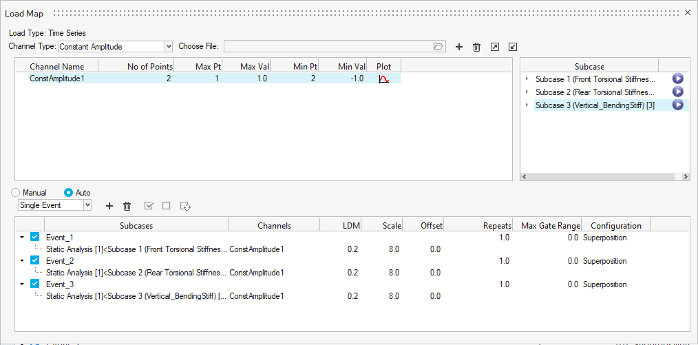
    The Load Map dialog opens.
  2. From the Channel Type drop-down menu at the top of the dialog, select Constant Amplitude.
  3. Click to add the load case.
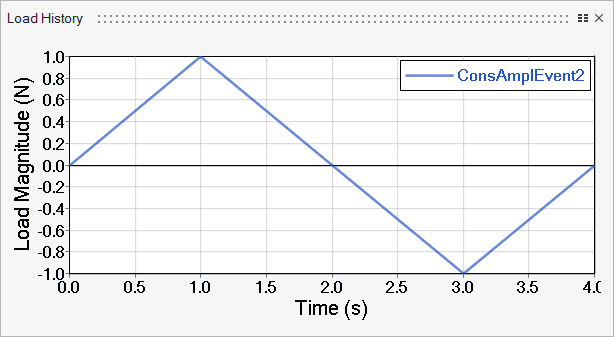
    Tip: Click to view a plot of the load.


    Figure 10.
  4. On the bottom half of the dialog, set the radio button to Auto for event creation and select Single Event from the drop-down menu.
    This option assists in automatically creating an event based on the subcase and channel selection.
  5. Select both Subcase 1 and ConsAmpEvent1 and click next to Single Event.
    An Event_1 header is created.
  6. Select Subcase 2 and ConsAmpEvent1 and click .
    An Event_2 header is created.
  7. In a similar manner, create an Event_3 header.
  8. Activate the checkboxes for all three events.
  9. Set LDM to 0.2, Scale to 8.0 and Offset to 0.0 for Subcase 1.
  10. Right click on the Scale and LDM fields for Subcase 1 and select Apply value to all events.


    Figure 11.
  11. Exit the dialog.

Evaluate and View Results

  1. From the Evaluate tool group, click the Run Analysis tool.


    Figure 12.
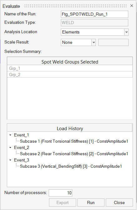
    The Evaluate dialog opens.


    Figure 13.
  2. Optional: Enter a name for the run.
  3. Click Run.
    Result files are saved to the home directory and the Run Status dialog opens.
  4. Once the run is complete, click View Current Results.
  5. Use the Results Explorer to visualize various types of results.


    Figure 14.


    Figure 15.

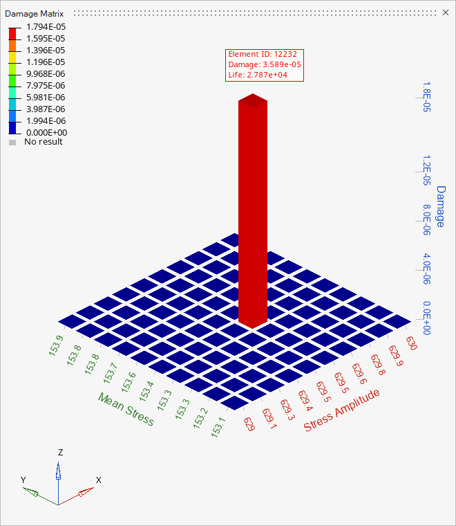
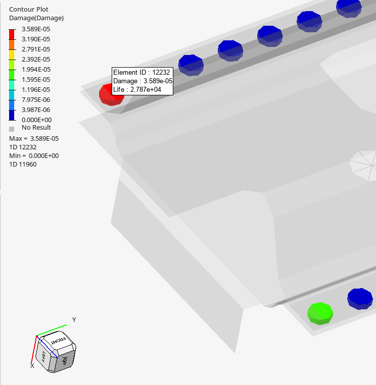
    The life of the critical spot weld is around 1.591e4 cycles.