OS-T: 5090 Thermal Optimization on Aluminum Fins

In this tutorial you will perform a shape optimization on an example of aluminum fins.
Before you begin, copy the file(s) used in this tutorial to your working directory.
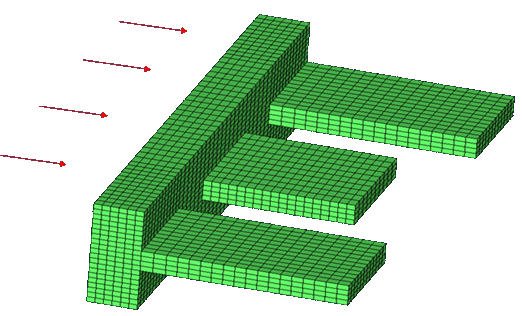
A part of the fins’ base experiences a constant heat flux of q=8000 W/m2. The temperature of the surrounding air is 283 K with a corresponding heat transfer coefficient of H = 40 W/m2 • K. The heat conduction coefficient is K = 221 W/m • K. The temperature distribution within the fins is determined by solving the heat conduction and convection load case.

os_5090_model
Figure 1. Model Overview
The formulation of the optimization problem is stated as:
Objective
Minimize the temperature at the center of the base.
Constraints
Volume < 1.0e-5 m2.
Design Variables
Shape design variables.

Launch HyperMesh and Set the OptiStruct User Profile

  1. Launch HyperMesh.
    The User Profile dialog opens.
  2. Select OptiStruct and click OK.
    This loads the user profile. It includes the appropriate template, macro menu, and import reader, paring down the functionality of HyperMesh to what is relevant for generating models for OptiStruct.

Import the Model

  1. Click File > Import > Solver Deck.
    An Import tab is added to your tab menu.
  2. For the File type, select OptiStruct.
  3. Select the Files icon files_panel.
    A Select OptiStruct file browser opens.
  4. Select the fins.fem file you saved to your working directory.
  5. Click Open.
  6. Click Import, then click Close to close the Import tab.

Set Up the Optimization

Create Shapes in HyperMorph

The Freehand module in HyperMorph creates the shapes.
  1. From the Analysis page, click the optimization panel.
  2. Click the HyperMorph panel.
  3. Click the Freehand panel.
  4. Select the move nodes subpanel.
  5. Set the movement option to translate.
  6. Input the translation distance.
    You only want to extend the fins in x-direction.
    1. In the x= field, enter 0.03.
    2. In the y= field, enter 0.0.
    3. In the z= field, enter 0.0.
  7. Select moving nodes.
    1. Under moving nodes, click nodes > by sets.
    2. Select sh1_move, then click select.
    The selected moving nodes are highlighted.
  8. Select fixed nodes.
    1. Under fixed nodes, click nodes > by sets.
    2. Select sh1_fix, then click select.
    The selected fixed nodes are highlighted.
  9. Select affected elements.
    1. Under affected elements, click elems > by sets.
    2. Select sh1_elem, then click select.
    The selected elements are highlighted.
  10. Click morph.
    The fin is extended in the x direction.
  11. Save the shape.
    1. Select the save shape subpanel.
    2. In the name= field, enter sh1.
    3. Toggle as handle perturbations to as node perturbations.
    4. Click save.
    The shape, sh1, for shape design variables is created.
  12. Click undo all.
  13. Repeat the above steps to create the shapes sh2 and sh3 on the original model. The corresponding node sets (sh2_move/fix and sh3_move/fix) and element sets (sh2_elem and sh3_elem) are predefined.
  14. Click return twice back to the Optimization panel.

Create Shape Design Variables

  1. Click the shape panel.
  2. Select the desvar subpanel.
  3. Switch from single desvar to multiple desvars.
  4. Using the shapes selector, select sh1, sh2, and sh3.
  5. In the initial value field, enter 0.0.
  6. In the lower bound field, enter -1.0.
  7. In the upper bound field, enter 2.0.
  8. Click create.
  9. Click return to go to the Optimization panel.
Three shape design variables are created from the shapes created in the previous step.

Create Optimization Responses

  1. From the Analysis page, click optimization.
  2. Click Responses.
  3. Create the volume response, which defines the volume fraction of the design space.
    1. In the responses= field, enter volume.
    2. Below response type, select volume.
    3. Set regional selection to total and no regionid.
    4. Click create.
  4. Create the temperature response.
    1. In the response= field, enter temperature.
    2. Set the response type to temperature.
    3. Click nodes > by id, then enter 2450 in the id= field.
    4. Click create.
    The temperature response at node 2450 is created.
  5. Click return to go back to the Optimization panel.

Create Design Constraints

  1. Click the dconstraints panel.
  2. In the constraint= field, enter vol.
  3. Click response = and select volume.
  4. Check the box next to upper bound, then enter 1.0e-5.
  5. Click create.
  6. Click return to go back to the Optimization panel.

Define the Objective Function

  1. Click the objective panel.
  2. Verify that min is selected.
  3. Click response and select temperature.
  4. Using the loadsteps selector, select heat transfer subcase.
  5. Click create.
  6. Click return twice to exit the Optimization panel.
The objective function of minimizing the temperature at node 2450 is created.

Define the SHAPE Card

Only displacement and stress results are available in the _s#.h3d file by default. To obtain analysis results (displacement/stress/temperature) on top of a shape change that was applied to the model in HyperView, a SHAPE card needs to be defined.
  1. From the Analysis page, click the control cards panel.
  2. In the Card Image dialog, click SHAPE.
  3. Set FORMAT to H3D.
  4. Set TYPE to ALL.
  5. Set OPTION to ALL.
  6. Click return twice to go back to the main menu.

Run the Optimization

  1. From the Analysis page, click OptiStruct.
  2. Click save as.
  3. In the Save As dialog, specify location to write the OptiStruct model file and enter fins_opt for filename.
    For OptiStruct input decks, .fem is the recommended extension.
  4. Click Save.
    The input file field displays the filename and location specified in the Save As dialog.
  5. Set the export options toggle to all.
  6. Set the run options toggle to optimization.
  7. Set the memory options toggle to memory default.
  8. Click OptiStruct to run the optimization.
    The following message appears in the window at the completion of the job:
    OPTIMIZATION HAS CONVERGED.
    FEASIBLE DESIGN (ALL CONSTRAINTS SATISFIED).
    OptiStruct also reports error messages if any exist. The file fins_opt.out can be opened in a text editor to find details regarding any errors. This file is written to the same directory as the .fem file.
  9. Click Close.

View the Results

The following steps demonstrate how to review the contour plot of the temperatures with the optimized shape in HyperView.
  1. In the OptiStruct panel, click HyperView.
  2. In the Load Results panel, load the fins_opt_s1.h3d file in both Model and Results fields.
  3. Click Apply.
    The .h3d file containing both the analysis and optimization results is loaded.
  4. In the Results Browser, select Iteration 0.
  5. On the Results toolbar, click resultsContour-16 to open the Contour panel.
  6. Set the Result type to Grid Temperatures (s).
  7. Click Apply.
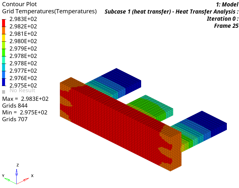
    The initial temperature distribution contour in the aluminum fins is displayed.
  8. In the Results Browser, select the last iteration.
  9. In the Contour panel, set the Result type to Shape Change (v).
  10. Click Apply.
    The optimized shape at final iteration is loaded.
  11. Set the Result type to Grid Temperatures (s).
  12. Click Apply.
The contour plot of grid temperature is applied on top of the optimized shape now.

os_5090_final
Figure 2. Temperature distribution of the original design
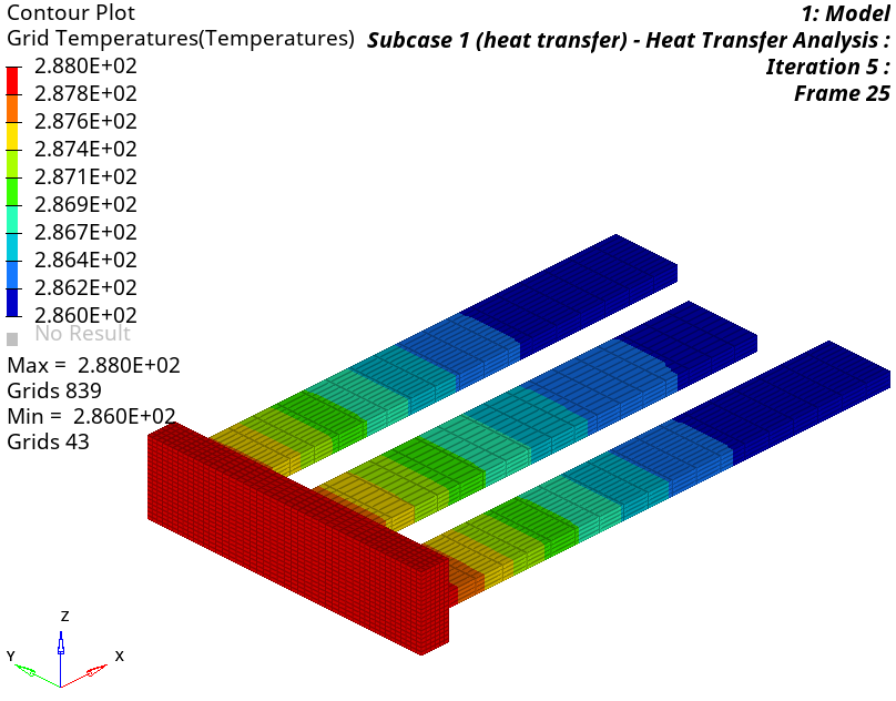

Figure 3. Temperature distribution in the optimized design