OS-HM-T: 6010 Fatigue Process Manager (FPM) using S-N (Stress - Life) Method
OptiStruct uses the S-N approach for calculating the fatigue life. The S-N approach is suitable for high cycle fatigue, where the material is subject to cyclical stresses that are predominantly within the elastic range. Structures under such stress ranges should typically survive more than 1000 cycles.
In OptiStruct various stress combination types are available, with the default being "Absolute maximum principle stress". In general "Absolute maximum principle stress" is recommended for brittle materials, while "Signed von Mises stress" is recommended for ductile material. The sign on the signed parameters is taken from the sign of the Maximum Absolute Principal value.
In this tutorial, you will be able to evaluate fatigue life with the S-N method through process manager step by step.
Launch Altair HyperWorks/HyperMesh and Process Manager
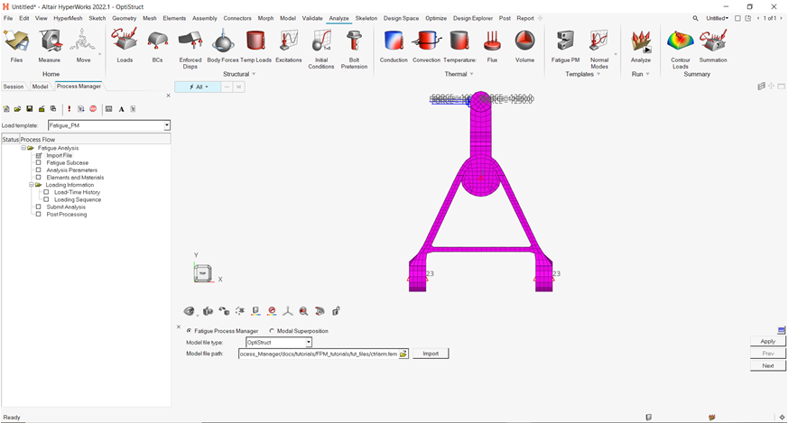
Import the Model
-
Click the Open model file icon
 .
A Select File browser window opens.
.
A Select File browser window opens. -
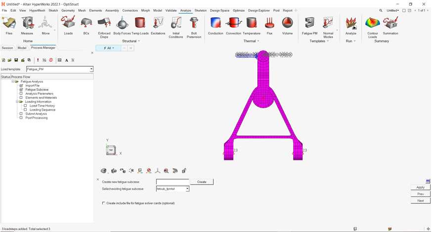
Click Apply.
This guides you to the next task Fatigue Subcase of the Fatigue Analysis tree.Figure 7. Import a Finite Element Model file
Set Up the Model
Create a Fatigue Subcase
-
Click Apply.
This saves the current definitions and guides you to the next task Analysis Parameters of the Fatigue Analysis tree.Figure 8. Create and Select Active Fatigue Subcase to Process
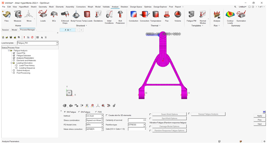
Apply Fatigue Analysis Parameters
-
Click Apply.
This saves the current definitions and guides you to the next task Elements and Materials of the Fatigue Analysis tree. For details, consult the Altair HyperWorks 2023 help.Figure 9. Fatigue Analysis Parameters Definition
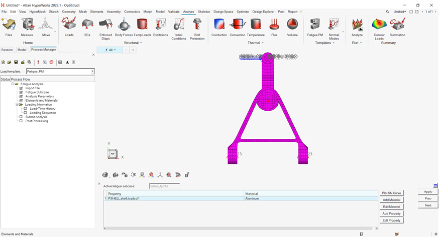
Add Fatigue Elements and Materials
-
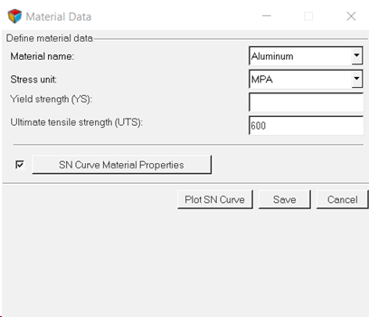
Click Add Material.
A Material Data window opens.Figure 10. Material Data Definition
-
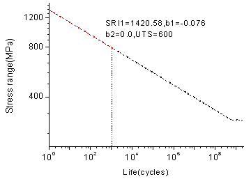
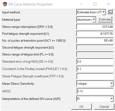
Click SN Curve Material Properties.
An SN Curve Material Properties dialog opens.Figure 11.
-
Click the Show SN curve definition icon
 .
An SN method description window introducing how to generate the SN material parameter opens.
.
An SN method description window introducing how to generate the SN material parameter opens. -
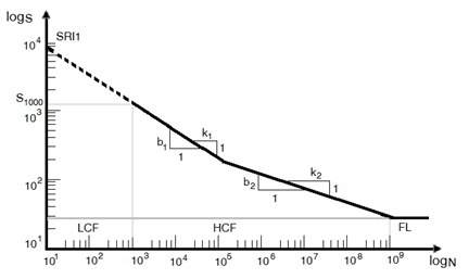
Click Plot SN Curve at the bottom of the window to show
the SN curve.
Figure 12.

-
Click Add Property.
A Property Data dialog opens.Figure 13.
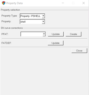
-
Click Close in the Property Data dialog to save the
fatigue definition.
This saves the current definitions and guides you to the next task Load-Time History of the Fatigue Analysis tree.Figure 14. Elements and Material Definition
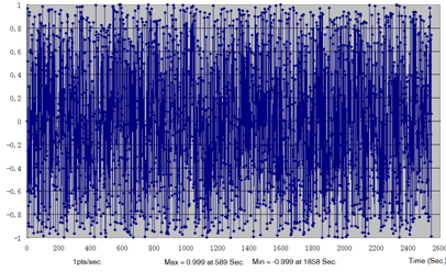
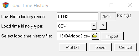
Apply Load-Time History
-
Click the Open load-time file icon .
An Open file browser window opens.
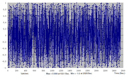
-
Create another load-time history LTH2 by importing the
file load2.csv.
Figure 15. Import Load-Time History
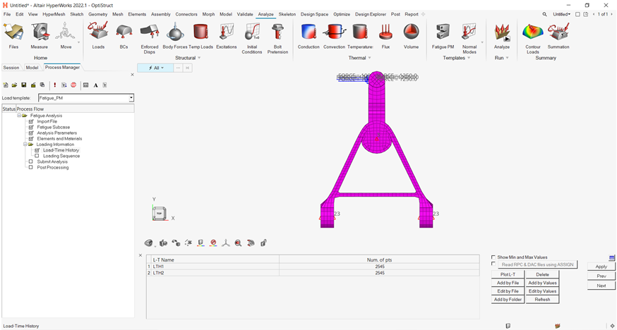
-
Click Apply.
This saves the current definitions and guides you to the next task Loading Sequences of the Fatigue Analysis tree.Figure 16. Load-Time History Definition
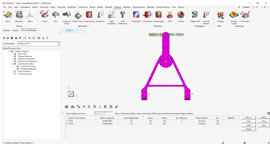
Load Sequences
-
Set Scale to 3.0, as shown below.
Figure 17. Load Mapping to associate load-time history with static subcase
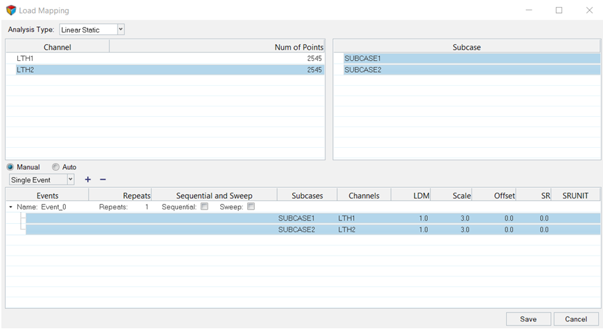
-
Click Save to close the window and create the fatique
event using selected subcases and channels.
Figure 18. Loading Sequences Definition
Submit the Job
-
Click the Save .fem file icon .
A Save As browser window opens.
-
Click Submit.
This launches OptiStruct 2023 to run the fatigue analysis. If the job is successful, the new results files should be in the directory from which ctrlarm_fpmtut.fem was selected.The default files written to the directory are:
ctrlarm_fpmtut.0.3.fat An ASCII format file which contains fatigue results of each fatigue subcase in iteration step. ctrlarm_fpmtut.h3d Hyper 3D binary results file, with both static analysis results and fatigue analysis results. ctrlarm_fpmtut.out OptiStruct output file containing specific information on the file set up, the set up of your fatigue problem, compute time information, etc. Review this file for warnings and errors. ctrlarm_fpmtut.stat Summary of analysis process, providing CPU information for each step during analysis process. Note: The filename.#.fat is created for each fatigue subcase at the first and last iterations only if a fatigue optimization is performed.Figure 19. Submit Fatigue Analysis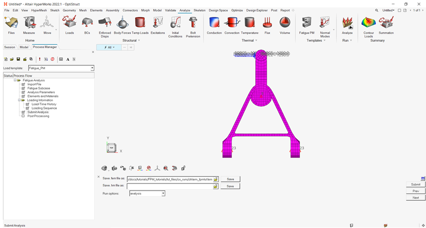 Figure 20.
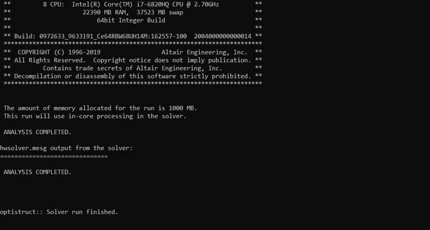
Post-process the Analysis
-
Click Exit to unload Fatigue Process Manager.
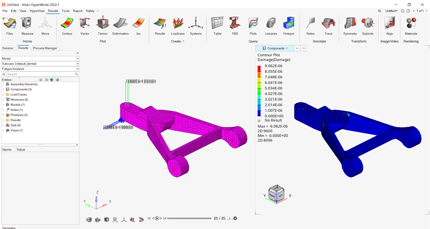
Figure 21. Post-Processing
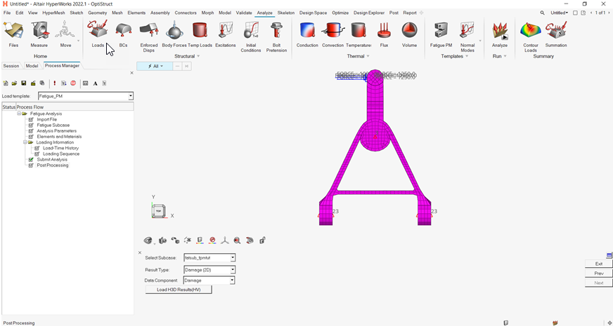 Figure 22. Damage Contour in HyperView