Smooth Implicit Geometry

Used to denoise objects created in Implicit Modeling. This reduces the size of, or removes, unwanted small and sharp features in an implicit body.

1. On the Implicit Modeling ribbon, select the Smooth tool.
   
   
2. Optional: For Visualization Quality, select from Low to Very High quality, which corresponds to a low to very high density of elements. A higher quality produces sharper geometry features but is more computationally intensive. When creating a complicated function, it’s recommended to work using a lower quality and then switch to a higher quality after the function is complete.
3. Select an implicit body to smooth.
4. Choose the Type of algorithm used to smooth the selected geometry.
   • Mean: The scalar value at each location is replaced with the mean value of all values in the kernel centered at that location in the field. This approach performs well in planar regions. However, it has a fillet-like effect on sharp edges, and it can introduce seams or other noise on curved surfaces that were not previously in the model. Please note that severe Mean smoothing can reduce the volume of the model and sometimes destroy thin or small features.
   • Median: The scalar value at each location is replaced by the median of all scalar values in the kernel centered at that location in the field. This smoothing type is particularly well-suited to removing "salt-and-pepper" or "impulse" noise, which are sharp and sudden disturbances in the field. This approach tends to perform well in planar regions. However, it has a chamfer-like effect on sharp edges, and it can introduce small seams on curved surfaces that were previously not in the model. The Median filter is relatively slow to compute as it is a non-linear rank filter, which requires the scalar values falling within the kernel to be sorted in order to compute the median value within the window.
   • Gaussian: Similar to the Mean approach, but neighboring values in the window (kernel) are given a different (lower) weighting than the scalar value at the center of the kernel, assigned using a Gaussian distribution. Rather than using the computationally slower true Gaussian distribution, we accurately approximate the Gaussian distribution by applying five consecutive iterations of a Mean filter (per iteration of the Gaussian smooth), which gives a very close approximation to the results of true Gaussian smoothing. This approach gives a good trade-off between localization and noise removal. However, it does not handle "salt-and-pepper" or "impulse" noise as well as the Median approach. Please note that severe Gaussian smoothing can reduce the volume of the model and sometimes destroy thin or small features.
   • Laplacian: This method uses the 7-point Discrete Laplacian kernel to smooth the scalar field. This is the most gentle of the smoothing operations, only marginally reducing the volume of the model with each iteration. Unlike other filters, Laplacian smoothing has to use more iterations to remove larger artifacts from the model.
5. Define the Width, which is the size of the smoothing kernel.
6. Define the Iterations, which are the number of times the smoothing kernel runs for.
7. Define the Strength, which morphs the smoothing results between 0% (no smoothing at all) and 100% (full-strength smoothing as per the Width and Iteration settings). The strength should be used to reduce the severity of the smoothing in delicate applications, such as those with this features. Further insights can be gained by referring Morph Implicit Geometry.
8. Click OK.
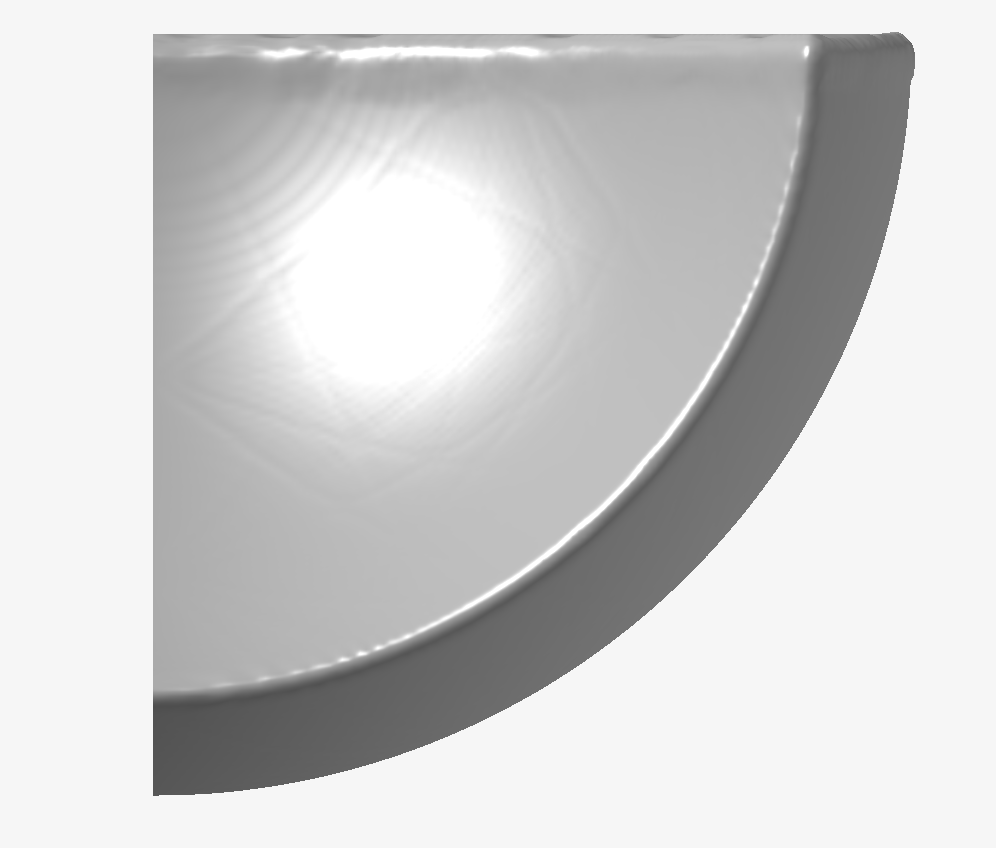
9. To give a visual demonstration of how different smoothing techniques impact Implicit Modeling geometry, the following images have been created using different smoothing kernels and different settings. Each image has a commentary that outlines the key observations in each case.
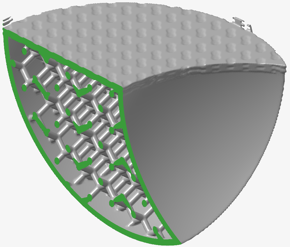
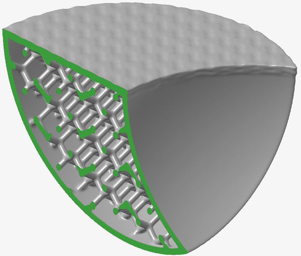
   To highlight the strengths and weaknesses of the different smoothing filters, the following test model has been constructed. It comprises spherical surfaces, a planar surface, an embedded strut lattice with fine details, and a deliberately poorly designed texture on the top face, leaving noisy artifacts in the model. As a result of some of the Boolean operations, areas of high curvature (somewhat sharp edges and corners) are also present in the model. The green coloring comes from using a section plane to reveal the lattice inside the object.

   
   
   

   Mean Smoothing

   Using a width of 1 (3 x 3 x 3 voxel kernel) and a single iteration:

   • Noisy artifacts removed from top face.
   • The texture depth and detail have both been reduced.
   • The noise along the sharper spherical edges has been reduced in a desirable manner.
   • Some spherical edges that we may have wished to remain sharp have been noticeably rounded.
   • The lattice struts are marginally thinner, but the junctions at the nodes and with the outer body have a noticeable fillet-like joint, which can be very useful for relieving stress raisers.

   
   
   

   Using a width of 1 (3 x 3 x 3 voxel kernel) and two iterations increases the severity of all of the effects outlined in the previous list of bullet points. There is further loss of detail in the texture, further rounding of sharp edges, and the struts of the lattices are thinner still.

   
   
   

   Interestingly, increasing the width of the kernel to two (5 x 5 x 5 voxel kernel) and using a single iteration is more severe than the previous example of using the same kernel with two iterations. In the image below, the struts in the lattice are thinner still, and the texture is almost completely lost.

   
   
   

   Finally, using a width of two and two iterations, the Mean smoothing starts to destroy struts in the lattice and the texture has practically disappeared.

   
   
   

   Median Smoothing

   Median smoothing is quite different from the other filters in terms of mathematical and computational composition. It is the only filter that ranks the values within the kernel, before selecting the middle value. It is therefore inherently non-linear. Using a kernel width of one and a single iteration, the following results are achieved:

   • Noisy artifacts removed from the top face.
   • The texture depth and detail have both been preserved (more than Mean smoothing).
   • The noise along the sharper spherical edges has been reduced in a desirable manner.
   • Some spherical edges that we may have wished to remain sharp are sharper than with Mean smoothing.
   • The lattice struts are marginally thinner, but the junctions at the nodes and with the outer body have a noticeable fillet-like joint, which can be very useful for relieving stress raisers.

   
   
   

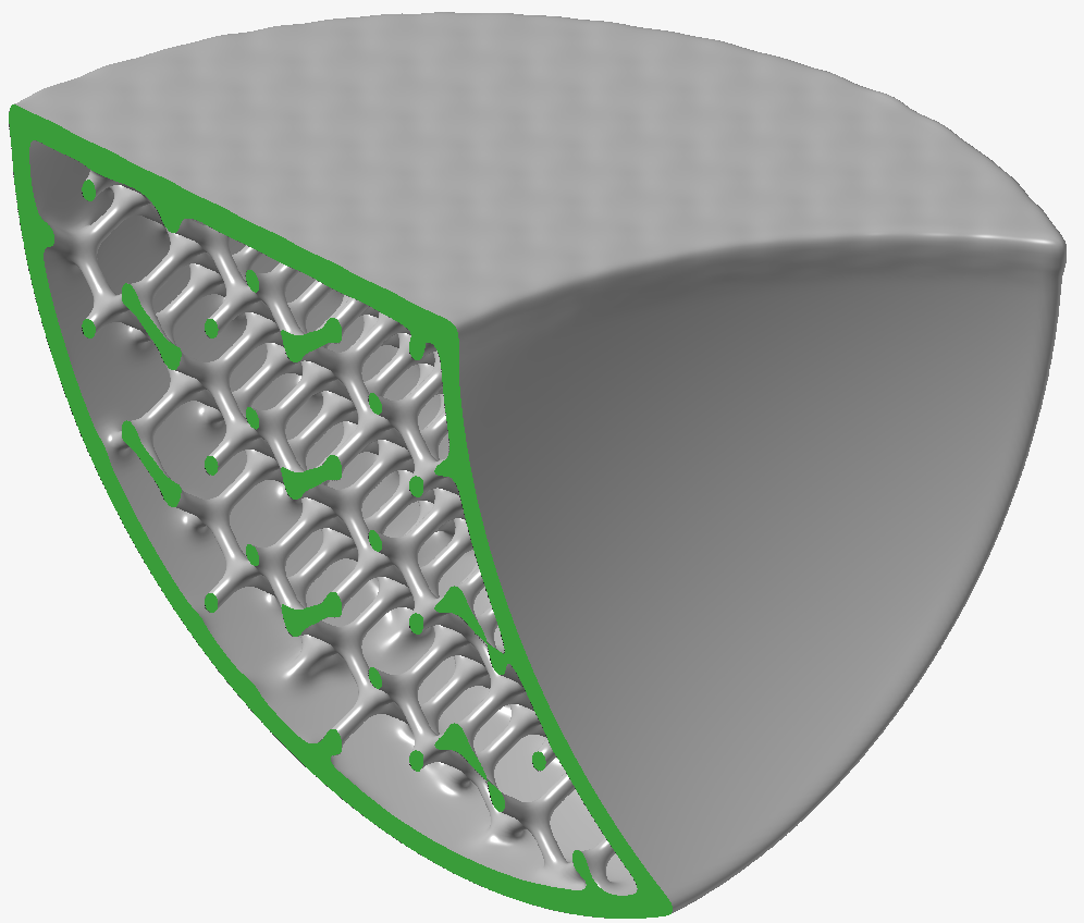
   It is sufficient to say that using a lower width with more iterations is generally less severe than using a larger width with fewer iterations. To show the more severe effects, the next image was created using a width of two and two iterations. The key observations are as follows:

   • The texture is clearly still visible.
   • The nodes of the lattice have been rounded, but the width of the struts in the lattice has been severely reduced. However, many of the struts are still visible, unlike when using the same settings on the Mean smoothing.
   • Some of the sharper edges have been rounded, whereas others are starting to present a chamfer-like effect.
   • The spherical surface is starting to exhibit straight-line patterning/texturing. This is a result of the non-linear nature of the smoothing filter. This is highlight from a different view in the second image below.

   
   
   

   
   
   

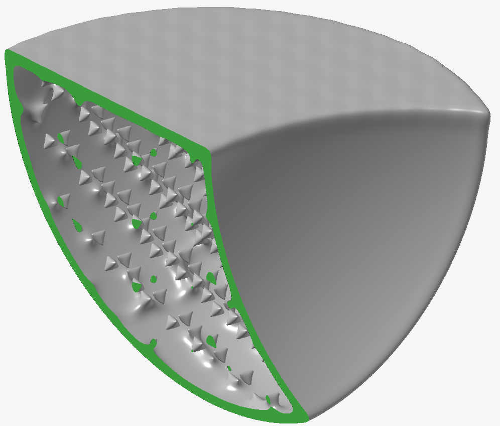
   Gaussian Smoothing

   In this implementation, a single iteration of Gaussian smoothing is approximated by running five consecutive iterations of Mean smoothing, which gives a very close approximation. As such, the attributes of Gaussian smoothing are largely in line with those for Mean smoothing with multiple iterations. However, as you might expect, Gaussian smoothing gives a somewhat harsh smoothing effect, reducing the thickness of fine features. The image below shows one iteration of Gaussian smoothing, which successfully removes noisy features and attractive blends have been created between the lattice and the outer body. In addition, some of the detail in the texture has been lost, sharp edges have been rounded, and some of the lattice struts have reduced in width.

   
   
   

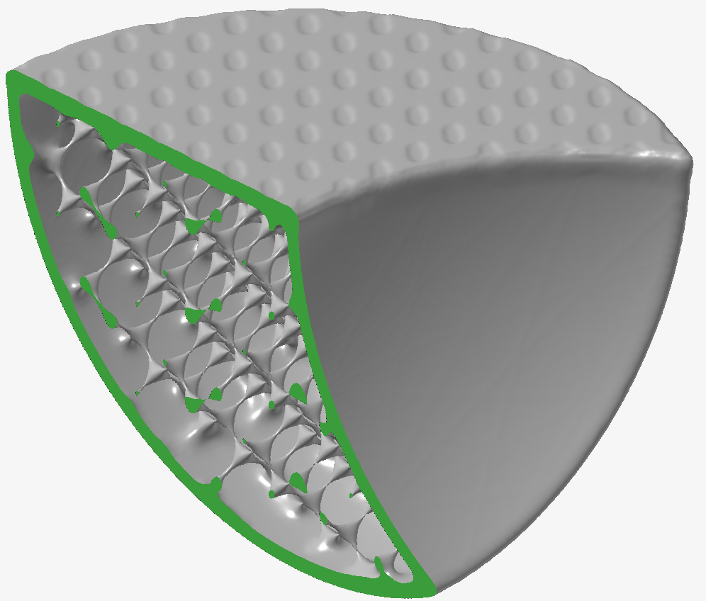
   Laplacian Smoothing

   Laplacian smoothing gives a gentler treatment than the other smoothing techniques. As such, more iterations are needed to remove larger artifacts. Although Laplacian smoothing does still reduce the thickness of the model, the fact that more iterations are needed gives a finer control over the balance between artifact removal and thickness preservation. The two images below were created using a width of one, and one (top) and nine (bottom) iterations, respectively. This gives you a feel for how gradual the smoothing and thinning effects are.