/FAIL/SYAZWAN

Block Format Keyword This simplified failure criterion is based on a fracture surface with linear damage accumulation. It also provides the initialization of damage value using strain histories with linear strain path assumptions.

Format

Card 1 – Fracture surface parameters 1

(1)	(2)	(3)	(4)	(5)	(6)	(7)	(8)	(9)	(10)
/FAIL/SYAZWAN/`mat_ID`/`unit_ID`
	$I c a r d$ $I c a r d$	$ε_{p}^{f}_{M I N}$ $ε_{p}^{f}_{M I N}$

I c a r d

$I c a r d$ = 1: classical input / Card 2 – Fracture surface parameters

(1)	(2)	(3)	(4)	(5)	(6)	(7)	(8)	(9)	(10)
`C`₁		`C`₂		`C`₃		`C`₄		`C`₅
`C`₆

I c a r d

$I c a r d$ = 2: plastic strain input / Card 2 – Failure plastic strains

(1)	(2)	(3)	(4)	(5)	(6)	(7)	(8)	(9)	(10)
$ε_{f}^{c o m p}$ $ε_{f}^{c o m p}$		$ε_{f}^{s h e a r}$ $ε_{f}^{s h e a r}$		$ε_{f}^{t e n s}$ $ε_{f}^{t e n s}$		$ε_{f}^{p l a n e}$ $ε_{f}^{p l a n e}$		$ε_{f}^{b i a x}$ $ε_{f}^{b i a x}$

Card 3 – Damage initialization parameters

(1)	(2)	(3)	(4)	(5)	(6)	(7)	(8)	(9)	(10)
	`D`_init	`D`_sf		`D`_max

Card 4 – Instability and softening parameters

(1)	(2)	(3)	(4)	(5)	(6)	(7)	(8)	(9)	(10)
`Inst`	`Iform`	`N`_value		`Soft`_exp

Card 5 – Element size scaling

(1)	(2)	(3)	(4)	(5)	(6)	(7)	(8)	(9)	(10)
	`fct_ID`_El	`El_ref`		`Fscale_El`

Card 6 - Optional line

(1)	(2)	(3)	(4)	(5)	(6)	(7)	(8)	(9)	(10)
`fail_ID`

Definition

Field	Contents	SI Unit Example
`mat_ID`	Material identifier. (Integer, maximum 10 digits)
`unit_ID`	(Optional) Unit identifier. (Integer, maximum 10 digits)
$I c a r d$ $I c a r d$	Card input format flag. 3 = 1 (Default) Fracture surface parameters input. = 2 Plastic strain at failure input. (Integer)
$ε_{p}^{f}_{M I N}$ $ε_{p}^{f}_{M I N}$	Minimum plastic strain at failure. Default = 0.0 (Real)
`C`₁	First constant for failure surface. (Real)
`C`₂	Second constant for failure surface. (Real)
`C`₃	Third constant for failure surface. (Real)
`C`₄	Fourth constant for failure surface. (Real)
`C`₅	Fifth constant for failure surface. (Real)
`C`₆	Sixth constant for failure surface. (Real)
$ε_{f}^{c o m p}$ $ε_{f}^{c o m p}$	Plastic strain at failure for uniaxial compression. (Real)
$ε_{f}^{s h e a r}$ $ε_{f}^{s h e a r}$	Plastic strain at failure for shearing. (Real)
$ε_{f}^{t e n s}$ $ε_{f}^{t e n s}$	Plastic strain at failure for uniaxial tension. (Real)
$ε_{f}^{p l a n e}$ $ε_{f}^{p l a n e}$	Plastic strain at failure for plane strain. (Real)
$ε_{f}^{b i a x}$ $ε_{f}^{b i a x}$	Plastic strain at failure for biaxial tension. (Real)
`D`_init	Damage value initialization from strain tensors flag. = 0 (Default) Damage is not initialized. = 1 Damage is initialized. (Integer)
`D`_sf	Damage initialization scale factor. Default = 1.0 (Real)
`D`_max	Damage initialization maximum value. Default = 1.0 (Real)
`Inst`	Necking instability flag. = 0 (Default) Instability is not activated. = 1 Instability is activated. (Integer)
`Iform`	Necking instability formulation flag. = 1 (Default) Incremental formulation (loading path history). = 2 Direct formulation (no loading path history). (Integer)
`N`_value	The N-value derived from Hollomon’s Law. Default = 0.25 (Real)
`Soft`_exp	Stress softening exponent. Default = 1.0 (Real)
`fct_ID`_El	Element size factor function identifier. (Integer)
`El_ref`	Reference element size. Default = 1.0 (Real)	$[m]$ $[m]$
`Fscale_El`	Element size factor function scale factor. Default = 1.0
`fail_ID`	(Optional) Failure criteria identifier. (Integer, maximum 10 digits)

▸Example

/FAIL/SYAZWAN/1
#              ICARD              EPFMIN
                   2                 0.0
#           EPF_COMP           EPF_SHEAR            EPF_TENS          EPF_PLSTRN            EPF_BIAX
               3.009                0.98                 0.7                0.42                0.56
#           DAM_INIT              DAM_SF             DAM_MAX
                   
#     INST     IFORM               N_VAL             SOFTEXP
         1         2                0.25                 1.2 
#             FCT_EL              EL_REF              ELSCAL                   

/FAIL/SYAZWAN/1
#              ICARD              EPFMIN
                   1                 0.0
#                 C1                  C2                  C3                  C4                  C5
                0.65             -3.2234               -0.08              3.9031              0.2652
#                 C6
              0.5266  
#           DAM_INIT              DAM_SF             DAM_MAX
                   
#     INST     IFORM               N_VAL             SOFTEXP
         1         1                0.27                 1.2 
#             FCT_EL              EL_REF              ELSCAL

Comments

It is highly recommended to set the value of $I_{p l a s}$ $I_{p l a s}$ in /PROP/SHELL to 1. This will allow accurate calculation of the principal strain ratio $β$ $β$ .
The value of C₁, C₂, C₃, C₄, C₅, and C₆ is based on:(1)
$ε_{p}^{f} = C_{1} + C_{2} η + C_{3} ¯ θ + C_{4} η^{2} + C_{5} {¯ θ}^{2} + C_{6} η ¯ θ$ $ε_{p}^{f} = C_{1} + C_{2} η + C_{3} \bar{θ} + C_{4} η^{2} + C_{5} {\bar{θ}}^{2} + C_{6} η \bar{θ}$

Where,

$ε_{p}^{f}$ $ε_{p}^{f}$

Plastic strain at failure.

$η$ $η$

Stress triaxiality with $η = \frac{\frac{1}{3} (σ_{x x} + σ_{y y})}{σ_{V M}}$ $η = \frac{\frac{1}{3} (σ_{x x} + σ_{y y})}{σ_{V M}}$

with $- \frac{2}{3} \leq η \leq \frac{2}{3}$ $- \frac{2}{3} \leq η \leq \frac{2}{3}$

$¯ θ$ $\bar{θ}$

Normalized Lode angle $¯ θ = 1 - \frac{2}{π} a r cos ζ$ $\bar{θ} = 1 - \frac{2}{π} a r \cos ζ$

with Lode angle ( $θ$ $θ$ ) parameter $ζ = cos (3 θ) = - \frac{27}{2} η (η^{2} - \frac{1}{3})$ $ζ = \cos (3 θ) = - \frac{27}{2} η (η^{2} - \frac{1}{3})$

Where, $σ_{V M}$ $σ_{V M}$ is the von Mises stress.

Figure 1 shows the example of curve fit of plane stress failure curve into failure surface criteria.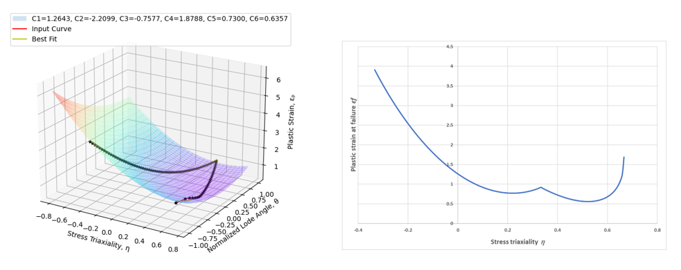

Figure 1. Example of Syazwan failure criterion fit
Two different parameter input card formats are available for /FAIL/SYAZWAN depending on the value of $I c a r d$ $I c a r d$ .
- If $I c a r d$ $I c a r d$ = 1: you must directly input the C_i parameters
- If $I c a r d$ $I c a r d$ = 2: you can specify some plastic strain at failure for several commonly tested loading conditions: uniaxial compression $ε_{f}^{c o m p}$ $ε_{f}^{c o m p}$ , shearing $ε_{f}^{s h e a r}$ $ε_{f}^{s h e a r}$ , uniaxial tension $ε_{f}^{t e n s}$ $ε_{f}^{t e n s}$ , plane strain $ε_{f}^{p l a n e}$ $ε_{f}^{p l a n e}$ and biaxial tension $ε_{f}^{b i a x}$ $ε_{f}^{b i a x}$ . In that case, the C_i parameter will be automatically computed by solving the set of equations below:(2)
  $⎧ ⎪ ⎪ ⎪ ⎪ ⎪ ⎪ ⎪ ⎪ ⎪ ⎪ ⎪ ⎪ ⎪ ⎪ ⎪ ⎨ ⎪ ⎪ ⎪ ⎪ ⎪ ⎪ ⎪ ⎪ ⎪ ⎪ ⎪ ⎪ ⎪ ⎪ ⎪ ⎩ \begin{matrix} C_{1} - \frac{1}{3} C_{2} - C_{3} + \frac{1}{9} C_{4} + C_{5} + \frac{1}{3} C_{6} = ε_{f}^{c o m p} C_{1} = ε_{f}^{s h e a r} C_{1} + \frac{1}{3} C_{2} + C_{3} + \frac{1}{9} C_{4} + C_{5} + \frac{1}{3} C_{6} = ε_{f}^{t e n s} C_{1} + \frac{1}{\sqrt{3}} C_{2} + \frac{1}{3} C_{4} = ε_{f}^{p l a n e} C_{1} + \frac{2}{3} C_{2} - C_{3} + \frac{4}{9} C_{4} + C_{5} - \frac{2}{3} C_{6} = ε_{f}^{b i a x} C_{2} - \frac{18}{π} C_{3} + \frac{2}{\sqrt{3}} C_{4} - \frac{18}{π \sqrt{3}} C_{6} = 0 \end{matrix}$ $\{\begin{cases} C_{1} - \frac{1}{3} C_{2} - C_{3} + \frac{1}{9} C_{4} + C_{5} + \frac{1}{3} C_{6} = ε_{f}^{c o m p} \\ C_{1} = ε_{f}^{s h e a r} \\ C_{1} + \frac{1}{3} C_{2} + C_{3} + \frac{1}{9} C_{4} + C_{5} + \frac{1}{3} C_{6} = ε_{f}^{t e n s} \\ C_{1} + \frac{1}{\sqrt{3}} C_{2} + \frac{1}{3} C_{4} = ε_{f}^{p l a n e} \\ C_{1} + \frac{2}{3} C_{2} - C_{3} + \frac{4}{9} C_{4} + C_{5} - \frac{2}{3} C_{6} = ε_{f}^{b i a x} \\ C_{2} - \frac{18}{π} C_{3} + \frac{2}{\sqrt{3}} C_{4} - \frac{18}{π \sqrt{3}} C_{6} = 0 \end{cases}$
Note: The last equation imposes that the plane strain condition corresponds to a local minimum of the failure criterion.
In some cases, the criterion may have negative or very low values for some loading conditions. In that case, it will be bounded by the minimum plastic strain at failure parameter $ε_{p}^{f}_{M I N}$ $ε_{p}^{f}_{M I N}$ that must be positive or null (by default = 0.0). All values under $ε_{p}^{f}_{M I N}$ $ε_{p}^{f}_{M I N}$ are then ignored.
Figure 2 shows an example with a minimum value (orange curve) of 0.2.

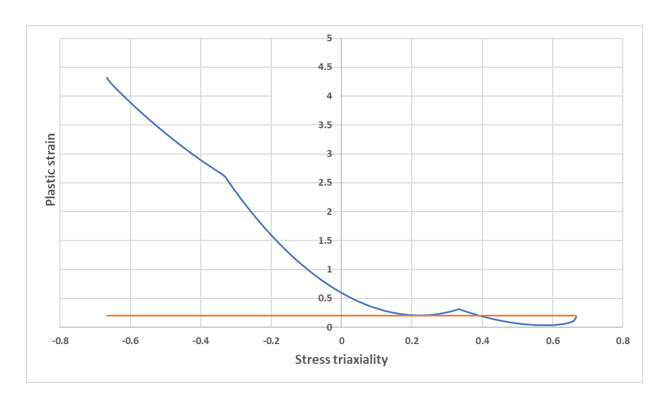
Figure 2. Failure criterion (blue curve) bounded by plastic strain at failure minimum value. $ε_{p}^{f}_{M I N}$ $ε_{p}^{f}_{M I N}$ (orange curve) of 0.2
The damage variable evolution is computed incrementally as:(3)
$D = \infty \sum t = 0 \frac{Δ ε_{p}}{ε_{p}^{f}}$ $D = \sum_{t = 0}^{\infty} \frac{Δ ε_{p}}{ε_{p}^{f}}$
You may want to realize a simulation starting from existing total and plastic strains fields (after a previous forming simulation for instance). In the case where the failure criterion is not computed during the first simulation, it is possible to estimate a damage field from the total strain tensor and the plastic strain values obtained at the end of the first simulation (using .sta files). If the D_init flag is set to 1, the damage field will be computed if the plastic strain ≠ 0. /INISHE/STRA_F, /INISHE/STRA_F, /INISHE/EPSP_F and /INISH3/EPSP_F must be present in the keywords of the status file. The initial stress tensors are not incorporated into the simulation model; thus, the stress triaxiality is derived using:(4)
$η = \frac{1}{\sqrt{3}} \frac{1 + β}{\sqrt{1 + β + β^{2}}}$ $η = \frac{1}{\sqrt{3}} \frac{1 + β}{\sqrt{1 + β + β^{2}}}$

The $β$ $β$ value can be recovered from the stress triaxiality value using the first root of Equation 4:(5)
$β = \frac{(2 - 3 η^{2}) - \sqrt{3 η^{2} (4 - 9 η^{2})}}{2 (3 η^{2} - 1)}$ $β = \frac{(2 - 3 η^{2}) - \sqrt{3 η^{2} (4 - 9 η^{2})}}{2 (3 η^{2} - 1)}$

Then, an initial damage value can be estimated as:(6)
$D_{t = 0} = \frac{ε_{p}^{t = 0}}{ε_{p}^{f}}$ $D_{t = 0} = \frac{ε_{p}^{t = 0}}{ε_{p}^{f}}$

Figure 3 shows an example of initialized damage field in one-step after a forming simulation performed without failure criterion computation. Damage field is then deduced using the plastic strain and the strain tensor as presented above.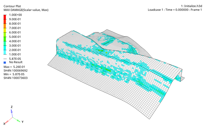

Figure 3. Example of damage field “one-step” initialization after a forming simulation
A controlled necking instability can be used if the flag Inst is set to 1. To trigger this instability, a criterion variable denoted $f$ $f$ is computed based on the N_value specified by you, using:(7)
$\begin{matrix} ε_{1} = \frac{2 (2 - α) (1 - α + α^{2})}{4 - 3 α - 3 α^{2} + 4 α} N_{v a l u e} ε_{2} = \frac{2 (2 α - 1) (1 - α + α^{2})}{4 - 3 α - 3 α^{2} + 4 α} N_{v a l u e} \end{matrix}$ $\begin{array}{l} ε_{1} = \frac{2 (2 - α) (1 - α + α^{2})}{4 - 3 α - 3 α^{2} + 4 α} N_{v a l u e} \\ ε_{2} = \frac{2 (2 α - 1) (1 - α + α^{2})}{4 - 3 α - 3 α^{2} + 4 α} N_{v a l u e} \end{array}$

Where, $α$ $α$ ratio between the minor principal and major principal stress computed from $β$ $β$ using:(8)
$α = \frac{2 β + 1}{2 + β}$ $α = \frac{2 β + 1}{2 + β}$

You can then compute an effective plastic strain at necking instability:(9)
$ε_{p}^{i n s t} = ε_{1} \cdot \sqrt{\frac{4}{3} (1 + β + β^{2})}$ $ε_{p}^{i n s t} = ε_{1} \cdot \sqrt{\frac{4}{3} (1 + β + β^{2})}$

The parameter N_value is the value of the instability plastic strain taken in uniaxial tension (for which $η = 1 / 3$ $η = 1 / 3$ and $¯ θ = 1$ $\bar{θ} = 1$ ). You can then use the relation linking $β$ $β$ and the stress triaxiality described above to plot the instability strain evolution.
Using the instability plastic strain, an instability criterion variable denoted $f$ $f$ is either computed:
- Incrementally (if Iform = 1) to take into account the loading history(10)
  $f = \infty \sum t = 0 \frac{Δ ε_{p}}{ε_{p}^{i n s t}}$ $f = \sum_{t = 0}^{\infty} \frac{Δ ε_{p}}{ε_{p}^{i n s t}}$
- Directly (if Iform = 2) to ignore the loading path history(11)
  $f = \frac{ε_{p}}{ε_{p}^{i n s t}}$ $f = \frac{ε_{p}}{ε_{p}^{i n s t}}$
If the criterion is reached ( $f = 1$ $f = 1$ ), the instant value of the damage variable $D$ $D$ is saved in the value $D_{c r i t}$ $D_{c r i t}$ that becomes an element history variable. The necking instability can then be triggered by a stress softening whose equation is:(12)
$\begin{matrix} D = \int Δ D f = \int Δ f D_{c r i t} = {\begin{matrix} \begin{matrix} 1 & while & f < 1 \end{matrix} \begin{matrix} D & when & f \geq 1 \end{matrix} \end{matrix} σ = σ_{e f f} (1 - {(\frac{D - D_{c r i t}}{1 - D_{c r i t}})}_{exp}^{S o f t_{exp}}) \end{matrix}$ $\begin{array}{l} D = \int Δ D \\ f = \int Δ f \\ D_{c r i t} = \{\begin{matrix} \begin{matrix} 1 & while & f < 1 \end{matrix} \\ \begin{matrix} D & when & f \geq 1 \end{matrix} \end{matrix} \\ σ = σ_{e f f} (1 - {(\frac{D - D_{c r i t}}{1 - D_{c r i t}})}^{S o f t_{\exp}}) \end{array}$

Where,

$σ$ $σ$

Damaged stress tensor.

$σ_{e f f}$ $σ_{e f f}$

Undamaged effective stress tensor.

$D_{c r i t}$ $D_{c r i t}$

Critical damage value that triggers stress softening.

$S o f t_{exp}$ $S o f t_{\exp}$

Exponent parameter.

For visualization purposes, the instability curve ( $ε_{p}^{i n s t}$ $ε_{p}^{i n s t}$ versus $η$ $η$ ) can be obtained from all the equations above. For instance, if the N_value is set to 0.175, the following curve (Figure 4) is obtained.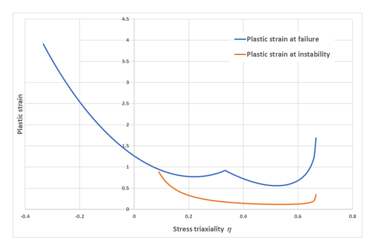

Figure 4. Example of instability curve (orange) and its position with respect to failure criterion (blue)

The effect of instability curve is restricted to positive stress triaxiality (as necking only occurs in tension) and only has an effect when it is under the failure criterion curve.

Figure 5 shows several instability curves obtained with different N_value parameter values.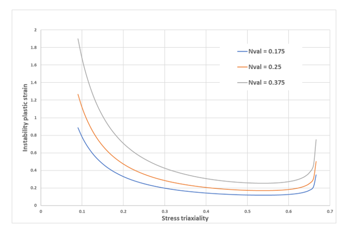

Figure 5. Instability curves obtained with different N_value parameters
Element size scaling can be used to regularize the failure and ensure to obtain an almost constant fracture energy dissipated with different mesh sizes. This element size dependency is introduced by computing a size scale factor denoted $f_{s i z e}$ $f_{s i z e}$ defined by the function fct_ID_El. The size scaling factor evolution is given with respect to the ratio of initial element characteristic length divided by a reference size El_ref (by default = 1.0): $f_{s i z e} (\frac{L_{e}^{0}}{L_{r e f}})$ $f_{s i z e} (\frac{L_{e}^{0}}{L_{r e f}})$ . An additional scale factor Fscale_El can also be applied to the entire regularization function. The element size scale factor $f_{s i z e}$ $f_{s i z e}$ thus computed is introduced in the damage variable evolution equation (and if defined, the instability variable evolution equation) as:(13)
$D = \infty \sum t = 0 \frac{Δ ε_{p}}{ε_{p}^{f} \cdot f_{s i z e} (\frac{L_{e}^{0}}{L_{r e f}}) \cdot f_{s c a l e}^{e l}}$ $D = \sum_{t = 0}^{\infty} \frac{Δ ε_{p}}{ε_{p}^{f} \cdot f_{s i z e} (\frac{L_{e}^{0}}{L_{r e f}}) \cdot f_{s c a l e}^{e l}}$
Alternatively, the /NONLOCAL/MAT option which is compatible with Syazwan failure criterion (Figure 6) can be used to regularize the solution according to mesh size and orientation. If the non-local regularization is used, the non-local plastic strain is used to compute the damage evolution (and the instability variable, if used). In that case, the maximum non-local length parameter LE_MAX is used instead of the initial element size if an element size scaling is defined through fct_ID_El. Also, the non-local regularization is also available with the “one-step” damage field initialization.

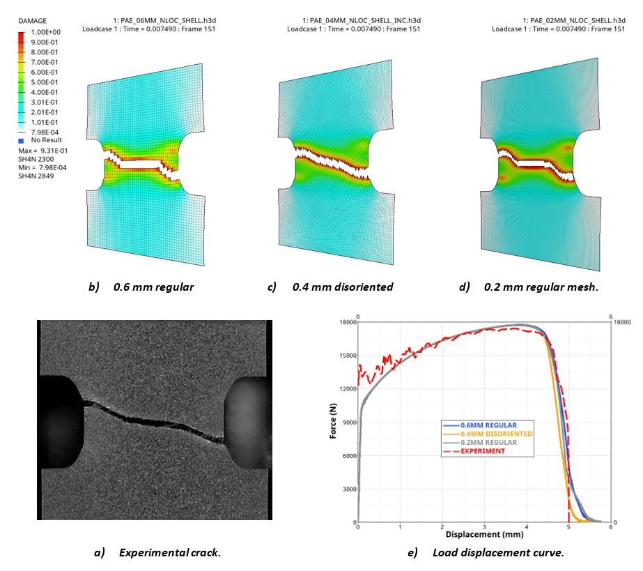
Figure 6. Example of /NONLOCAL/MAT option cumulated with /FAIL/SYAZWAN on automotive DP450 steel