RD-E: 5600 Hyperelastic Material with Curve Input
The target of this example is to demonstrate how to use material test data for rubber hyperplastic materials.
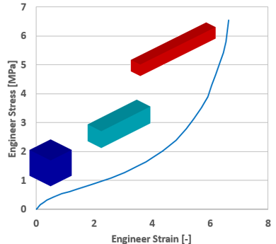
Figure 1.
Options and Keywords Used
- Ogden material law /MAT/LAW42 (OGDEN)
- /MAT/LAW62 (VISC_HYP)
- /MAT/LAW69
- /MAT/LAW82
- /MAT/LAW88
- Arruda-Boyce material law /MAT/LAW92
- Yeoh material law /MAT/LAW94 (YEOH)
Input Files
Model Description
Uniaxial tensile one brick element with imposed displacement and fixed in other side only in X direction.
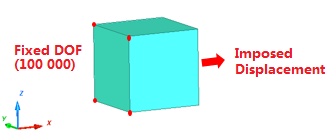
Figure 2. Problem Description
Units: mm, s, Mg, N, MPa
Table 1 shows curve input or parameter input available for hyperelastic material model.
Properties: /PROP/SOLID with, Isolid=24, Ismstr=10, and Icpre=1.
When using hyperelastic material laws, there are some recommended element property settings. When using solid elements, it is always better to mesh with 8 node /BRICK elements if possible. If not then /TETRA4 or /TETRA10 elements can be used.
- Ismstr=10
- Icpre=1 with Isolid=24.
Simulation Iterations
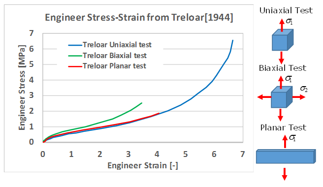
Figure 3. Test Data from Treloar [1944]
| Material Law | Test Data Input | Parameter Input | |
|---|---|---|---|
| Ogden | LAW42 | √ | |
| LAW62 | √ | ||
| LAW69 | √ | ||
| LAW82 | √ | ||
| LAW88 | √ | ||
| Arruda-Boyce | LAW92 | √ | √ |
| Yeoh | LAW94 | √ |
For the Ogden based laws, LAW69 will be used to curve fit the test data and extract material parameters that can be used in LAW42, LAW62, and LAW82. Next the test data will be used in LAW88 and LAW92. Finally, a fitting script will be used to extract the LAW94 material parameters.
Results
Ogden Model
- Uniaxial engineering compressive stain
- Equal biaxial engineering tension strain
- Uniaxial engineering compressive stress
- Equal biaxial engineering tension stress
The engineering strain should be monotonically increasing going from a negative value in compression to a positive value in tension. In compression, the engineering strain should not be less than -1.0 since -100% strain is physically not possible. Fitting test data that represents the anticipated strain state of material will give the most accurate material parameters for a particular situation. Although a tension only uniaxial stress strain curve could be used, this example uses uniaxial compression and tension data to better fit for both compressive and tension loading conditions.
- Number of material parameter () pairs: N=2 or 3. (N > 3 is rarely used)
- Engineering stress-strain curve from uniaxial compression/tension test set in fct_ID1
- : This value is to get the best fit for the incompressible rubber material but as described later, this high value causes a low time step and thus a value of 0.495 is typically recommended.
After running the Radioss Starter, the output file (*0000.out) contains the stress strain curve for the calculated material fit parameters and the original input data. The calculated fitted parameters, shear modulus, and bulk modulus are also included in the output.
    FITTING RESULT COMPARISON:

      UNIAXIAL TEST DATA

      NOMINAL STRAIN     NOMINAL STRESS(TEST)       NOMINAL STRESS(RADIOSS)
           -0.9495           -221.4526                   -220.7771
           -0.9449           -176.9213                   -175.8148
           -0.9396           -138.1769                   -139.3528
           -0.9289            -93.5350                    -93.1405
           -0.9150            -60.3881                    -61.2494
           -0.8911            -35.8292                    -35.2551
           -0.8387            -15.4000                    -15.5512
           -0.7343             -5.7900                     -5.7761
           -0.6457             -3.1912                     -3.2391
           -0.5041             -1.5128                     -1.5510
           -0.4173             -1.0147                     -1.0297
           -0.3056             -0.5855                     -0.5989
           .......             .......                    ........
-------------------------------------------
AVERAGED ERROR OF FITTING :       2.00%


     FITTED PARAMETERS FOR HYPERELASTIC_MATERIAL LAW
      ----------------------------------------
     OGDEN LAW PARAMETERS:
     MU1 . . . . . . . . . . . . . . . . . .=-0.2397367723469
     MU2 . . . . . . . . . . . . . . . . . .= -11.57584346215
     MU3 . . . . . . . . . . . . . . . . . .=  11.57477242242
     MU4 . . . . . . . . . . . . . . . . . .=  0.000000000000
     MU5 . . . . . . . . . . . . . . . . . .=  0.000000000000

     AL1 . . . . . . . . . . . . . . . . . .= -4.548308811208
     AL2 . . . . . . . . . . . . . . . . . .=  5.714056272418
     AL3 . . . . . . . . . . . . . . . . . .=  5.714110104590
     AL4 . . . . . . . . . . . . . . . . . .=  0.000000000000
     AL5 . . . . . . . . . . . . . . . . . .=  0.000000000000

     GROUND-STATE SHEAR MODULE . . . . . . .= 0.5424499939537
     BULK MODULUS. . . . . . . . . . . . . .=  903.9025065914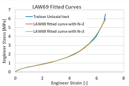
Figure 4. LAW69 Fitted Curve with N=2 and N=3 for Odgen Model
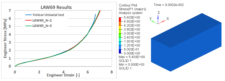
Figure 5. LAW69 Results from a 1 Element Model with N=2 and N=3
Figure 5 shows the calculated stress strain curve from the 1 element model simulation matches the Treloar test data.
The engineering stress strain curves were calculated from the true stress and true strain in principal direction 1 (P1) from the animation output /ANIM/BRICK/TENS/STRAIN and /ANIM/BRICK/TENS/STRESS using these formulas.
,
,
The effect of different Poison’s ratio input can be seen in Figure 6. The largest difference in the results is at higher amounts of strain. The results will match the test data better when but this results in a time step that is 4 times lower than . Thus, to balance the computation time and accuracy it is recommended to use for incompressible rubber material.
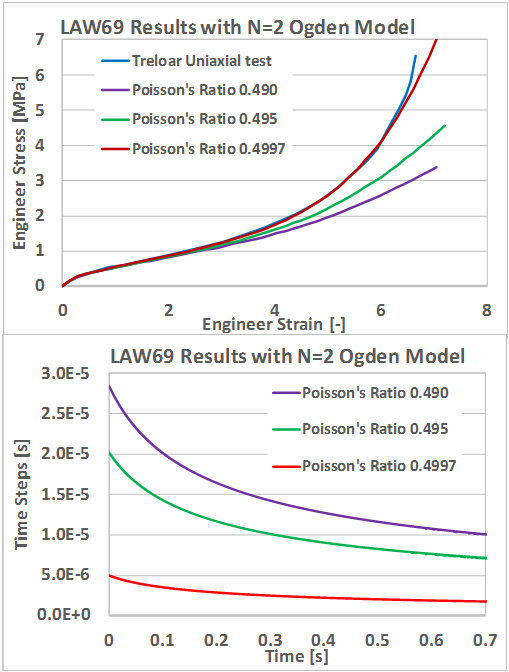
Figure 6. Effect of Poisson’s Ratio in Results and in Time Step
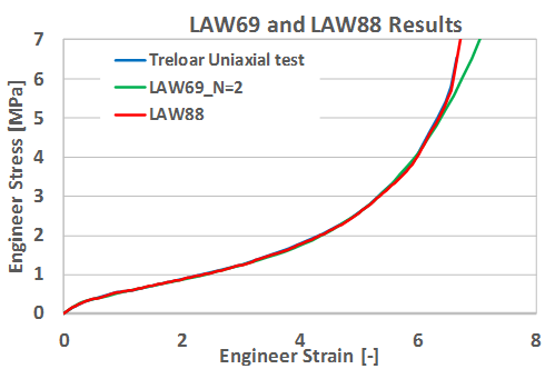
Figure 7. Results of LAW69 and LAW88 Compared with Test Data
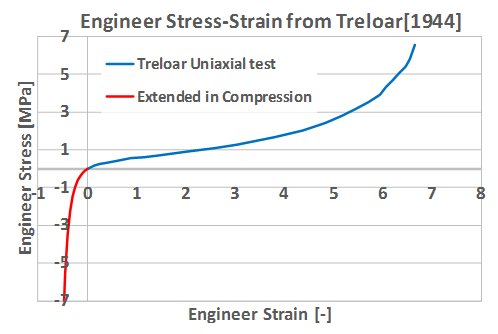
Figure 8. Test Data Extended in Compression
- For LAW42, the LAW69 fitted Ogden parameters can be taken from the
Starter output and used as input in LAW42.LAW42
(4) - For LAW62 and LAW82, the Ogden parameters need to be converted from
LAW69 fitted Ogden parameters because the Ogden model equation is
different in LAW62 and LAW82.
Considering an Ogden model with N=2, the energy density function used in LAW42 and LAW82 are shown here for an incompressible material.
LAW62 (and LAW82)(5)
- LAW62
- LAW82
Figure 9 shows the material fit parameters from LAW69 converted into LAW82 match the LAW69 and LAW42 results for Ogden order, N=2.
#RADIOSS STARTER
/UNIT/1
UNIT FOR MAT
                  Mg                  mm                   s
#---1----|----2----|----3----|----4----|----5----|----6----|----7----|----8----|----9----|---10----|
#---1----|----2----|----3----|----4----|----5----|----6----|----7----|----8----|----9----|---10----|
/MAT/OGDEN/1/1
rubber LAW42
#              RHO_I
                1E-9
#                 Nu           sigma_cut           funIDbulk         Fscale_bulk         M     Iform
               .4997                   0                   0                   0         0         0
#               Mu_1                Mu_2                Mu_3                Mu_4                Mu_5
 1.2732565785698E-05    -0.2635330119696                   0                   0                   0
# blank card

#            alpha_1             alpha_2             alpha_3             alpha_4             alpha_5
      7.168617832124     -4.158214786551                   0                   0                   0
# blank card

#---1----|----2----|----3----|----4----|----5----|----6----|----7----|----8----|----9----|---10----|
#enddata#RADIOSS STARTER
#---1----|----2----|----3----|----4----|----5----|----6----|----7----|----8----|----9----|---10----|
/MAT/LAW82/1
rubber LAW82
# RHO_I
1E-9 0
# N Nu
2 .4997
# Mu_i
0.000045637449070023 0.547913433558156 0 0 0
# Alpha_i
7.168617832124 -4.158214786551 0 0 0
# D_i
0 0
#---1----|----2----|----3----|----4----|----5----|----6----|----7----|----8----|----9----|---10----|
#enddata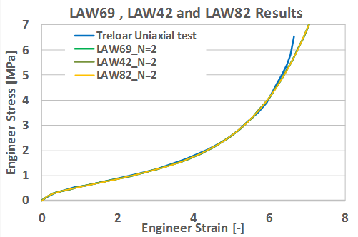
Figure 9. Results of LAW69, LAW42 and LAW82 Compared with Test Data
Arruda-Boyce Model
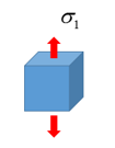
Figure 10. Itype=1: Uniaxial test
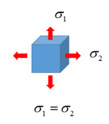
Figure 11. Itype=2: Equibiaxial test
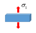
Figure 12. Itype=3: Planar test
In LAW92, if the curve input is used then the parameter lines can be left blank. Only one type of test data type can be considered at a time.
#RADIOSS STARTER
#-  2. MATERIALS:
/UNIT/1
UNIT FOR MAT
                  Mg                  mm                   s
#---1----|----2----|----3----|----4----|----5----|----6----|----7----|----8----|----9----|---10----|
#---1----|----2----|----3----|----4----|----5----|----6----|----7----|----8----|----9----|---10----|
/MAT/LAW92/1/1
rubber
#              RHO_I
            1.000E-9
#                 mu                   D                 LAM
                   0                   0                   0
#    IType    fct_ID                  NU
         1         3               .4997
#---1----|----2----|----3----|----4----|----5----|----6----|----7----|----8----|----9----|---10----|
#ENDDATA
#---1----|----2----|----3----|----4----|----5----|----6----|----7----|----8----|----9----|---10----|-------------------------------------------
AVERAGED ERROR OF FITTING : 12.72%
FITTED PARAMETERS FOR HYPERELASTIC_MATERIAL LAW
----------------------------------------
ARRUDA-BOYCE LAW
MU . . . . . . . . . . . . . . . . . . . .= 0.3023683957840
D. . . . . . . . . . . . . . . . . . . . .= 3.8695518555789E-03
LAM. . . . . . . . . . . . . . . . . . . .= 4.917777266862
GROUND-STATE SHEAR MODULE. . . . . . . . .= 0.3101754654817
BULK MODULUS . . . . . . . . . . . . . . .= 516.8557173143When the Radioss Engine is ran, the fitted Arruda-Boyce parameters are used to compute the stress-strain behavior in hyperelastic material. Therefore, if the above fitted Arruda-Boyce parameter are used as LAW92 input, the results will be the same.
#RADIOSS STARTER
#-  2. MATERIALS:
/UNIT/1
UNIT FOR MAT
                  Mg                  mm                   s
#---1----|----2----|----3----|----4----|----5----|----6----|----7----|----8----|----9----|---10----|
#---1----|----2----|----3----|----4----|----5----|----6----|----7----|----8----|----9----|---10----|
/MAT/LAW92/1/1
rubber
#              RHO_I
            1.000E-9
#                 mu                   D                 LAM
     0.3023683957840 3.8695518555789E-03      4.917777266862
#    IType    fct_ID                  NU

#---1----|----2----|----3----|----4----|----5----|----6----|----7----|----8----|----9----|---10----|
#ENDDATA
#---1----|----2----|----3----|----4----|----5----|----6----|----7----|----8----|----9----|---10----|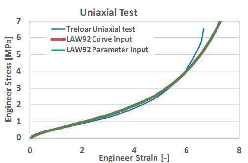
Figure 13. Equivalent LAW92 Used with Curve Input and Parameter Input
- Fitted in LAW92 Curve Input
- 6.4695283364675E-02
- 3.8695518555789E-03
Yeoh Model
Since the Yeoh model only depends on , only the uniaxial test is needed to calculate the Yeoh material parameters. Here are the stretch in principal direction 1, 2, 3 and . is the engineer strain in principal direction .
Uniaxial Test
and
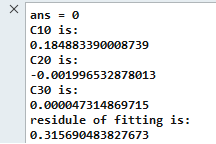
Figure 14. Fitted Yeoh Parameter with Compose Script
Next, the curve fit values can be used in LAW94 and the results compared to the original test data. In the example, you have been using to get a good fit to the test data. can then be calculated from .
Where, .
#---1----|----2----|----3----|----4----|----5----|----6----|----7----|----8----|----9----|---10----|
/MAT/LAW94/1
plastic
#              RHO_I
              1.0E-9
#Blank

#                C10                 C20                 C30
   0.184883390008739  -0.001996532878013   0.000047314869715
#                 D1                  D2                  D3
   0.003245938015181
#---1----|----2----|----3----|----4----|----5----|----6----|----7----|----8----|----9----|---10----|
#ENDDATA
#---1----|----2----|----3----|----4----|----5----|----6----|----7----|----8----|----9----|---10----|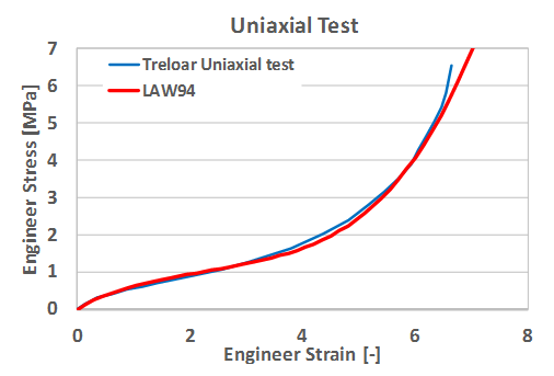
Figure 15. Results of LAW94 with Fitted Yeoh Parameter
References
http://www.axelproducts.com/downloads/TestingForHyperelastic.pdf